Chapter 8 Text Analysis

Evgeny Klochikhin and Jordan Boyd-Graber

This chapter provides an overview of how social scientists can make use of text data using computational data analysis methods. We cover the types of analysis that can be done with text data (search, topic detection, classification, etc.) and give an overview of how to do these analyses, social science tasks that they’re useful for, and how to evaluate the results produced. We also provide pointers to some tools that are commonly used for doing text analysis.

8.1 Understanding human generated text

As social scientists, we often deal with text data that comes from a variety of sources: open ended survey responses, phone call transcriptions, social media data, notes from electronic health records, news articles, and research publications. A challenge we face when dealing with these types of data is how to efficiently analyze them just like we analyze traditional tabular data.

For example, when analyzing survey responses or electronic health records data, both of which contain narrative text (from the respondents and medical practitioners, respectively), the text data often gets ignored or selectively read by the analysts (manually) and used anecdotally. Text analysis techniques described in this chapter allow you to use all of the data available (structured and unstructured), and incorporate large amounts of text data in your analysis.

8.2 How is text data different than “structured” data?

We’re often comfortable analyzing ‘’structured data’’ that is organized as rows and columns. Text data, often also known as unstructured data⁶³, is harder to analyze using traditional data analysis tools because it doesn’t come as a set of rows and columns, but instead consists of characters, words, sentences, and paragraphs. In traditional, “structured” data, a human has already decided what constitutes a row (a person, for example), what constitutes a column (their age, sex, address, for example), and the relationship between them. We covered that in the Database chapter where we created a data model for a given domain. When dealing with text data, we have to create the tabular ourselves.

While creating that tabular structure, we have to deal with human language being complex and nuanced which makes automatically analyzing it difficult. We often make simplifying assumptions: we assume our input is clean text; we ignore humor (Halevy, Norvig, and Pereira 2009) and deception (Niculae et al. 2015; Ott et al. 2011); and we assume “standard” English (Kong et al. 2014)⁶⁴. Text data also often reflects human observations that are exceptions to regular processes: e.g., the ubiquitous “other” or the “anything else you want to tell us” field in questionnaires. Recognizing this complexity, the goal of text analysis is to efficiently extract important information from large amounts of text, and use it for/in our analysis just like we use tabular data.

8.3 What can we do with text data?

There are a lot of types of analysis that we can do with text data. Table 8.1 gives a summary of these types of analysis.⁶⁵

Table 8.1: Text analysis examples
Type of Analysis	Description	Examples
Search	Finding relevant content based on some information need, often specified as a set of keywords/phrases but can be more structured.	For example, we used these techniques in systematic literature reviews to facilitate the discovery and retrieval of relevant publications related to early grade reading in Latin America and the Caribbean.
Topic Detection / Clustering	Used to explore and understand what types of words, phrases, and topics exist in text data.	Given thousands of e-mails from a corporation, characterize the broad themes that are prominent in the firm’s communication.
Classification	Used to classify text content into one or more predefined categories.	Given SMS messages from a disaster region, decide whether the sender needs medical assistance, food, or shelter (Yates and Paquette 2010).
Sentiment analysis	Detection of sentiment or opinions at different levels of granularity—document, paragraph/sentence or entity (person, organization, etc.) level.	Examples using machine learning to analyze the flow and topic segmentation of political debates and behaviors (Nguyen, Boyd-Graber, and Resnik 2012; Nguyen et al. 2015) and to assign automated tags to documents (Tuarob, Pouchard, and Giles 2013).
Word Clustering/Synonyms	Finding groups of words that are similar to each other. Depending on the problem need, similarity can be defined as strictly synonyms or aliases (such as IBM and Big Blue being synonyms in a specific context).	In a search engine, when a user searches for “Russian astronaut”, also return search results for “Soviet cosmonaut” (Zeng et al. 2012).
Named Entity Linking	Recognition, tagging and extraction of named entities (typically of type Person, Location, Organization) from text data. Typically limited to proper nouns.	Given an e-mail, automatically link all of the names to their corresponding Wikipedia page (Ferragina and Scaiella 2010).
General Extraction	Recognition, tagging, and extraction of specific classes of words/phrases that may be entities, events, relationships between entities, etc.	Automatically detecting words as types of events (holiday, party, graduation for example) and classifying them into types (related to sports, politics, and religion for example) from tweets (Ritter et al. 2012).
Visualization	Visualization of text data and/or visual mashups combining text with other forms of data (such as maps or networks).	Given grants funded by the NIH, create a visualization to find areas where directorates could collaborate with each other (Talley et al. 2011).
Summarization	Summarization of a document (or a set of documents), either as a set of important keywords, or important sentences extracted from the text, or new sentences generated to produce a summary.	For example, Wang et al. (2009) use topic modeling to produce category-sensitive text summaries and annotations on large-scale document collections.
Translation	Automatic translation of text from one language to another.	Look at reaction to a political event in newspapers of different countries in different languages.

For this chapter, we will focus on two types of use cases that social scientists deal with containing text data:

Content understanding: We have some text “corpus”, for example open-ended survey responses or news articles or research publications, and our goal is to understand the content—patterns, themes, trends—of that data. This often involves methods from unsupervised machine learning (that we covered in the previous chapter). The analysis can then be combined with tabular data that might accompany the text. For example, the survey responses may also have structured information that the respondent filled out, or the news article or research publication has meta-data that can be augmented with information generated from the text analysis.
Content Classification: The second use case is less focused on “discovery” and “understanding new content” and instead focuses on efficiently classifying content into a pre-defined set of categories. The text data is similar to the previous use case but the task is different, and can often be a follow-up task to the previous use case. We might have news articles about politics that we need to automatically classify into issue areas that are being discussed such as healthcare, education, foreign policy, etc. Another example is analyzing research publications that we need to classify into topics or research areas. This falls into supervised learning in the machine learning framework that we covered in the previous chapter.

8.4 How to analyze text

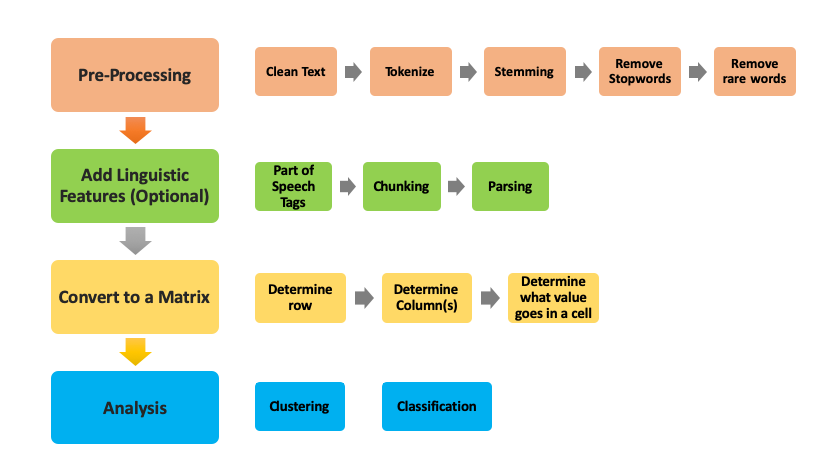
Text analysis, specially related to the clustering and classification use cases, requires us to build an analysis pipeline that processes data through a series of steps:

Initial Processing: We take raw text data (word documents, html content scraped from webpages, etc.) and run it through some initial processing where the goal is to clean the text (dealing with content that is redundant or dirty, such as cleaning up html if processing data from web pages), turning sentences or documents into words or phrases, or removing words that we don’t consider useful for a specific analysis.
Adding Linguistic Features: This step is only needed when the problem requires deeper linguistic analysis. For example, when trying to understand the structure of a sentence, we can augment the raw words with their part-of-speech tags using a part-of-speech tagger for deeper analysis. Or use a statistical parser to generate what’s called a parse tree that shows relationships between different components of a sentence.
Converting the enriched text to a matrix: Once we’ve cleaned up the text data and split them into sentences, phrases, words, and their corresponding linguistic attributes, the goal of this step is to make decisions that turn our “document” into a matrix. The key decisions in this step we have to make are 1) defining what a row is, 2) defining what a column is, and 3) what do we put as the value for a cell in a given row and column.
Analysis: Once we have a matrix, then we can apply the methods we covered in the previous chapter (such as clustering and classification) as well as any other data analysis methods available to us. Later in this chapter, we’ll go deeper into applying these methods to text data as well as describe new methods that are specifically designed for text analysis.

8.4.1 Initial Processing

The first important step in working with text data is cleaning and processing.⁶⁶ Textual data are often messy and unstructured, which makes many researchers and practitioners overlook their value. Depending on the source, cleaning and processing these data can require varying amounts of effort but typically involve a set of established techniques.

Tokenization

The first step in processing text is deciding what terms and phrases are meaningful. Tokenization separates sentences and terms from each other. The Natural Language Toolkit (NLTK) (Bird, Klein, and Loper 2009) provides simple reference implementations of standard natural language processing algorithms such as tokenization—for example, sentences are separated from each other using punctuation such as period, question mark, or exclamation mark. However, this does not cover all cases such as quotes, abbreviations, or informal communication on social media. While separating sentences in a single language is hard enough, some documents “code-switch” (Molina et al. 2016), combining multiple languages in a single document. These complexities are best addressed through data-driven machine learning frameworks (Kiss and Strunk 2006).

Stop words

Once the tokens are clearly separated, it is possible to perform further text processing at a more granular, token level. Stop words are a category of words that have limited semantic meaning (and hence utility) regardless of the document content. Such words can be prepositions, articles, common nouns, etc. For example, the word “the” accounts for about 7% of all words in the Brown Corpus, and “to” and “of” are more than 3% each (Malmkjær 2002). We may choose to remove stopwords if we think that they won’t be useful in our analysis. For example, words such as “the”, “is”, “or” may not be useful if the task is to classify news articles into the topic of the article. On the other hand, they may provide information information if the task is to classify a document into the genre it belongs to or in identifying the author of the document.

In addition to removing frequent words, it often helps to remove words that only appear a few times. These words—names, misspellings, or rare technical terms—are also unlikely to bear significant contextual meaning. Similar to stop words, these tokens are often disregarded in further modeling either by the design of the method or by manual removal from the corpus before the actual analysis.

\(N\)-grams

However, individual words are sometimes not the correct unit of analysis. For example, blindly removing stop words can obscure important phrases such as “systems of innovation,” “cease and desist,” or “commander in chief.” Identifying these \(N\)-grams requires looking for statistical patterns to discover phrases that often appear together in fixed patterns (Dunning 1993). These combinations of phrases are often called collocations, as their overall meaning is more than the sum of their parts. N-grams can be created over any unit of analysis, such as sequences of characters (called character n-grams) or sequences of phonemes that are used in speech recognition.

Stemming and lemmatization

Text normalization is another important aspect of preprocessing textual data. Given the complexity of natural language, words can take multiple forms dependent on the syntactic structure with limited change of their original meaning. For example, the word “system” morphologically has a plural “systems” or an adjective “systematic.” All these words are semantically similar and—for many tasks—should be treated the same. For example, if a document has the word “system” occurring three times, “systems” once, and “systematic” twice, one can assume that the word “system” with similar meaning and morphological structure can cover all instances and that variance should be reduced to “system” with six instances.

The process for text normalization is often implemented using established lemmatization and stemming algorithms. A lemma is the original dictionary form of a word. For example, “go,” “went,” and “goes” will all have the lemma “go.” The stem is a central part of a given word bearing its primary semantic meaning and uniting a group of similar lexical units. For example, the words “order” and “ordering” will have the same stem “ord.” Morphy (a lemmatizer provided by the electronic dictionary WordNet), Lancaster Stemmer, and Snowball Stemmer are common tools used to derive lemmas and stems for tokens, and all have implementations in the NLTK (Bird, Klein, and Loper 2009).

8.4.2 Linguistic Analysis

So far, we’ve treated words as tokens without regard to the meaning of the word or the way it is used, or even what language the word comes from. There are several techniques in text analysis that are language-specific that go deeper into the syntax of the document, paragraph, and sentence structure to extract linguistic characteristics of the document.

Part-of-speech tagging

When the examples \(x\) are individual words and the labels \(y\) represent the grammatical function of a word (e.g., whether a word is a noun, verb, or adjective), the task is called part-of-speech tagging. This level of analysis can be useful for discovering simple patterns in text: distinguishing between when “hit” is used as a noun (a Hollywood hit) and when “hit” is used as a verb (the car hit the guard rail).

Unlike document classification, the examples \(x\) are not independent: knowing whether the previous word was an adjective makes it far more likely that the next word will be a noun than a verb. Thus, the classification algorithms need to incorporate structure into the decisions. Two traditional algorithms for this problem are hidden Markov models (Rabiner 1989) and conditional random fields (Lafferty, McCallum, and Pereira 2001), but more complicated models have higher accuracy (Plank, Søgaard, and Goldberg 2016).

Order Matters

All text-processing steps are critical to successful analysis. Some of them bear more importance than others, depending on the specific application, research questions, and properties of the corpus. Having all these tools ready is imperative to producing a clean input for subsequent modeling and analysis. Some simple rules should be followed to prevent typical errors. For example, stop words should not be removed before performing \(n\)-gram indexing, and a stemmer should not be used where data are complex and require accounting for all possible forms and meanings of words. Reviewing interim results at every stage of the process can be helpful.

8.4.3 Turning text data into a matrix: How much is a word worth?

The processing stages described above provide us with the columns in our matrix. Now we have to decide how to assign values in that column for each word or phrase. In text analysis, we typically refer to them as tokens (where a token can be a word or a phrase). One simple approach would be to give each column a binary 0 or 1 value—if this token occurs in a document, we assign that cell a value of 1 and 0 otherwise. Another approach would be to assign it the value of how many times this token occurs in that document (often known as frequency of that term or token). This is essentially a way to define the importance or value of this token in this document. Not all words are worth the same; in an article about sociology, “social” may be less important or informative than “inequality”. Appropriately weighting⁶⁷ and calibrating words is important for both human and machine consumers of text data: humans do not want to see “the” as the most frequent word of every document in summaries, and classification algorithms benefit from knowing which features are actually important to making a decision.

Weighting words requires balancing how often a word appears in a local context (such as a document) with how much it appears overall in the document collection. Term frequency–inverse document frequency (TFIDF) (Salton 1968) is a weighting scheme to explicitly balance these factors and prioritize the most meaningful words. The TFIDF model takes into account both the term frequency of a given token and its document frequency (Box TFIDF) so that if a highly frequent word also appears in almost all documents, its meaning for the specific context of the corpus is negligible. Stop words are a good example when highly frequent words also bear limited meaning since they appear in virtually all documents of a given corpus.

Box: TFIDF

For every token \(t\) and every document \(d\) in the corpus \(D\) of size \(\mid D\mid = N\), TFIDF is calculated as \[tfidf(t,d,D) = tf(t,d) \times idf(t,D),\] where term frequency is either a simple count, \[tf(t,d)=f(t,d),\] or a more balanced quantity, \[tf(t,d) = 0.5+\frac{0.5 \times f(t,d)}{\max\{f(t,d):t\in d\}},\] and inverse document frequency is \[\ idf(t,D) = \log\frac{N}{|\{d\in D:t\in d\}|}.\]

8.4.4 Analysis

Now that we have a matrix with documents as rows, words/phrases as columns, and let’s say the TFIDF score as the value of that word in that document, we are now ready to run different machine learning methods on this data. We will not recap all of the methods and evaluation methodologies already covered in Chapter Machine Learning here but they can all be used with text data.

We’ll focus on three types of analysis: finding similar documents, clustering, and classification. For each type of analysis, we‘ll focus on what it allows us to do, what types of tasks social scientists will find it useful for, and how to evaluate the results of the analysis.

Use Case: Finding Similar Documents

One task social scientists may be interested in is finding similar documents to a document they’re analyzing. This is a routine task during literature review where we may have a paper and we’re interested in finding similar papers or in disciplines such as law, where lawyers looking at a case file want to find all prior cases related to the case being reviewed. The key challenge here is to define what makes two documents similar - what similarity metrics should we use to calculate this similarity? Two commonly used metrics are Cosine Similarity and Kullback–Leibler divergence (Kullback and Leibler 1951).

Cosine similarity is a popular measure in text analysis. Given two documents \(d_a\) and \(d_b\), this measure first turns the documents into vectors (each dimension of the vector can be a word or phrase) \(\overrightarrow{t_a}\) and \(\overrightarrow{t_b}\), and uses the cosine similarity (the cosine of the angle between the two vectors) as a measure of their similarity. This is defined as:

\[SIM_C(\overrightarrow{t_a},\overrightarrow{t_b}) = \frac{\overrightarrow{t_a} \cdot \overrightarrow{t_b}}{|\overrightarrow{t_a}|\times|\overrightarrow{t_b}|}.\]

Kullback–Leibler (KL) divergence is a measure that allows us to compare probability distributions in general and is often used to compare two documents represented as vectors. Given two term vectors \(\overrightarrow{t_a}\) and \(\overrightarrow{t_b}\), the KL divergence from vector \(\overrightarrow{t_a}\) to \(\overrightarrow{t_b}\) is \[D_{KL}(\overrightarrow{t_a}||\overrightarrow{t_b}) = \sum\limits_{t=1}^m w_{t,a}\times \log\left(\frac{w_{t,a}}{w_{t,b}}\right),\] where \(w_{t,a}\) and \(w_{t,b}\) are term weights in the two vectors, respectively, for terms \(t=1, \ldots, m\).

An averaged KL divergence metric is then defined as \[D_{AvgKL}(\overrightarrow{t_a}||\overrightarrow{t_b}) = \sum\limits_{t=1}^m (\pi_1\times D(w_{t,a}||w_t)+\pi_2\times D(w_{t,b}||w_t)),\] where \(\pi_1 = \frac{w_{t,a}}{w_{t,a}+w_{t,b}}, \pi_2 = \frac{w_{t,b}}{w_{t,a}+w_{t,b}}\), and \(w_t = \pi_1\times w_{t,a} + \pi_2\times w_{t,b}\) (Huang 2008).

A Python-based scikit-learn library provides an implementation of these measures as well as other machine learning models and approaches

Example: Measuring similarity between documents

NSF awards are not labeled by scientific field—they are labeled by program. This administrative classification is not always useful to assess the effects of certain funding mechanisms on disciplines and scientific communities. A common need is to understand how awards are similar to each other even if they were funded by different programs. Cosine similarity allows us to do just that.

Example code

The Python numpy module is a powerful library of tools for efficient linear algebra computation. Among other things, it can be used to compute the cosine similarity of two documents represented by numeric vectors, as described above. The gensim module that is often used as a Python-based topic modeling implementation can be used to produce vector space representations of textual data.

Augmenting Similarity Calculations with External Knowledge repositories

It’s often the case that two, especially short, documents do not have any words in common but are still similar. In such cases, cosine similarity or KL divergence do not help us with the similarity calculations without augmenting the data with additional information. Often, external data resources that provide relationships between words, documents, or concepts present in specific domains can be used to achieve that. Established corpora, such as the Brown Corpus and Lancaster–Oslo–Bergen Corpus, are one type of such preprocessed repositories.

Wikipedia and WordNet are examples of another type of lexical and semantic resources that are dynamic in nature and that can provide a valuable basis for consistent and salient information retrieval and clustering. These repositories have the innate hierarchy, or ontology, of words (and concepts) that are explicitly linked to each other either by inter-document links (Wikipedia) or by the inherent structure of the repository (WordNet). In Wikipedia, concepts thus can be considered as titles of individual Wikipedia pages and the contents of these pages can be considered as their extended semantic representation.

Information retrieval techniques build on these advantages of WordNet and Wikipedia. For example, Meij et al. (2009) mapped search queries to the DBpedia ontology (derived from Wikipedia topics and their relationships), and found that this mapping enriches the search queries with additional context and concept relationships. One way of using these ontologies is to retrieve a predefined list of Wikipedia pages that would match a specific taxonomy. For example, scientific disciplines are an established way of tagging documents—some are in physics, others in chemistry, engineering, or computer science. If a user retrieves four Wikipedia pages on “Physics”, “Chemistry”, “Engineering”, and “Computer Science”, they can be further mapped to a given set of scientific documents to label and classify them, such as a corpus of award abstracts from the US National Science Foundation.

Personalized PageRank is a similarity system that can help with the task. This system uses WordNet to assess semantic relationships and relevance between a search query (document \(d\)) and possible results (the most similar Wikipedia article or articles). This system has been applied to text categorization (Navigli et al. 2011) by comparing documents to semantic model vectors of Wikipedia pages constructed using WordNet. These vectors account for the term frequency and their relative importance given their place in the WordNet hierarchy, so that the overall \(wiki\) vector is defined as:

\[SMV_{wiki}(s) = \sum\nolimits_{w\in Synonyms(s)} \frac{tf_{wiki}(w)}{|Synsets(w)|}\],

where \(w\) is a token (word) within \(wiki\), \(s\) is a WordNet synset (a set of synonyms that share a common meaning) that is associated with every token \(w\) in WordNet hierarchy, \(Synonyms(s)\) is the set of words (i.e., synonyms) in the synset \(s\), \(tf_{wiki}(w)\) is the term frequency of the word \(w\) in the Wikipedia article \(wiki\), and \(Synsets(w)\) is the set of synsets for the word \(w\).

The overall probability of a candidate document \(d\) (e.g., an NSF award abstract or a PhD dissertation abstract) matching the target query, or in our case a Wikipedia article \(wiki\), is \[wiki_{BEST}=\sum\nolimits_{w_t\in d} \max_{s\in Synsets(w_t)} SMV_{wiki}(s),\] where \(Synsets(w_t)\) is the set of synsets for the word \(w_t\) in the target document document (e.g., NSF award abstract) and \(SMV_{wiki}(s)\) is the semantic model vector of a Wikipedia page, as defined above.

Evaluating “Find Similar” Methods

When developing methods to find similar documents, we want to make sure that we find all relevant documents that are similar to the document under consideration, and we want to make sure we don’t find any non-relevant documents. Chapter Machine Learning already touched on the importance of precision and recall for evaluating the results of machine learning models (Box Precision and recall provides a reminder of the formulae). The same metrics can be used to evaluate the two goals we have in finding relevant and similar documents.

Box: Precision and recall

Precision computes the type I errors—false positives (retrieved documents that are not relevant)—and is formally defined as \[\mathrm{Precision} = \frac{|\{\mathrm{relevant\ documents}\}\cap \{\mathrm{retrieved\ documents}\}|}{|\{\mathrm{retrieved\ documents}\}|}.\] Recall accounts for type II errors—false negatives (relevant documents that were not retrieved)—and is defined as \[\mathrm{Recall}=\frac{|\{\mathrm{relevant\ documents}\}\cap \{\mathrm{retrieved\ documents}\}|}{|\{\mathrm{relevant\ documents}\}|}.\]

We assume that a user has three sets of documents \(D_a =\{d_{a1},d_{a2},\ldots, d_n\}\), \(D_b=\{d_{b1}, d_{b2}, \ldots, d_k\}\), and \(D_c =\{d_{c1},d_{c2},\ldots,d_i\}\). All three sets are clearly tagged with a disciplinary label: \(D_a\) are computer science documents, \(D_b\) are physics, and \(D_c\) are chemistry.

The user also has a different set of documents—Wikipedia pages on “Computer Science,” “Chemistry,” and “Physics.” Knowing that all documents in \(D_a\), \(D_b\), and \(D_c\) have clear disciplinary assignments, let us map the given Wikipedia pages to all documents within those three sets. For example, the Wikipedia-based query on “Computer Science” should return all computer science documents and none in physics or chemistry. So, if the query based on the “Computer Science” Wikipedia page returns only 50% of all computer science documents, then 50% of the relevant documents are lost: the recall is 0.5.

On the other hand, if the same “Computer Science” query returns 50% of all computer science documents but also 20% of the physics documents and 50% of the chemistry documents, then all of the physics and chemistry documents returned are false positives. Assuming that all document sets are of equal size, so that \(|D_a| = 10\), \(|D_b|=10\) and \(|D_c| = 10\), then the precision is \(\frac{5}{12} = 0.42\).

F score

The F score or F1 score combines precision and recall. In formal terms, the \(F\) score is the harmonic mean of precision and recall: \[\label{eq:text:F1} F_1 = 2\cdot \frac{\mathrm{Precision}\cdot \mathrm{Recall}}{\mathrm{Precision}+\mathrm{Recall}}.\] In terms of type I and type II errors: \[F_\beta = \frac{(1+\beta^2)\cdot \mathrm{true\ positive}}{(1+\beta^2)\cdot \mathrm{true\ positive} + \beta^2\cdot \mathrm{false\ negative} + \mathrm{false\ positive}},\] where \(\beta\) is the balance between precision and recall. Thus, \(F_2\) puts more emphasis on the recall measure and \(F_{0.5}\) puts more emphasis on precision.

Examples

Some examples from our recent work can demonstrate how Wikipedia-based labeling and labeled LDA (Ramage et al. 2009; Nguyen et al. 2014) cope with the task of document classification and labeling in the scientific domain. See Table 8.2.

Table 8.2: Wikipedia articles as potential labels generated by \(n\)-gram indexing of NSF awards
Abstract excerpt	ProQuest subject category	Labeled LDA	Wikipedia-based labeling
Reconfigurable computing platform for smallscale resource-constrained robot. Specific applications often require robots of small size for reasons such as costs, access, and stealth. Smallscale robots impose constraints on resources such as power or space for modules…	Engineering, Electronics and Electrical; Engineering, Robotics	Motor controller	Robotics, Robot, Fieldprogrammable gate array
Genetic mechanisms of thalamic nuclei specification and the influence of thalamocortical axons in regulating neocortical area formation. Sensory information from the periphery is essential for all animal species to learn, adapt, and survive in their environment. The thalamus, a critical structure in the diencephalon, receives sensory information…	Biology, Neurobiology	HSD2 neurons	Sonic hedgehog, Induced stem cell, Nervous system
Poetry ’n acts: The cultural politics of twentieth century American poets’ theater. This study focuses on the disciplinary blind spot that obscures the productive overlap between poetry and dramatic theater and prevents us from seeing the cultural work that this combination can perform…	Literature, American; Theater	Audience	Counterculture of the 1960s, Novel, Modernism

Use Case: Clustering

Another task social scientists often perform is finding themes, topics, and patterns in a text data set, such as open-ended survey responses, news articles, or publications. Given open-ended responses from a survey on how people feel about a certain issue, we may be interested in finding out the common themes that occur in these responses. Clustering methods are designed to do exactly that. With text data, clustering is often used to explore what topics and concepts are present in a new corpus (collection of documents). It is important to note that if we already have a pre-specified set of categories and documents that are tagged with those categories, and the goal is to tag new documents, then we would use classification methods instead of clustering methods. As we covered in the previous chapter, clustering a is a form of unsupervised learning where the goal is exploration and understanding of the data.

As we covered earlier, unsupervised analysis of large text corpora without extensive investment of time provides additional opportunities for social scientists and policymakers to gain insights into policy and research questions through text analysis. The clustering methods described in the Machine Learning chapter, such as k-means clustering, can be used for text data as well once the text has been converted to a matrix as described earlier. We will describe Topic Modeling, that provides us with another clustering approach specifically designed for text data.

8.4.5 Topic modeling

Topic modeling is an approach that describes topics that constitute the high-level themes of a text corpus. Topic modeling is often described as an information discovery process: describing what “concepts” are present in a corpus. We refer to them as “concepts” or “topics” (in quotes) because they typically will be represented as a probability distribution over the words (that the topic modeling method groups together) which may or may not be semantically coherent as a “topic” to social scientists.

As topic modeling is a broad subfield of natural language processing and machine learning, we will restrict our focus to a single method called Latent Dirichlet Allocation (LDA) (Blei, Ng, and Jordan 2003). LDA is a fully Bayesian extension of probabilistic latent semantic indexing (Hofmann 1999), itself a probabilistic extension of latent semantic analysis (Landauer and Dumais 1997). Blei and Lafferty (2009) provide a more detailed discussion of the history of topic models.

LDA, like all topic models, assumes that there are topics that form the building blocks of a corpus. Topics are distributions over words and are often shown as a ranked list of words, with the highest probability words at the top of the list (see Figure 8.1). However, we do not know what the topics are a priori; the goal is to discover what they are (more on this shortly).

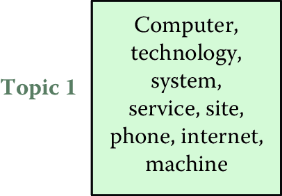
Topics are distributions over words. Here are three example topics learned by latent Dirichlet allocation from a model with 50 topics discovered from the *New York Times* [@sandhaus-08]. Topic 1 appears to be about technology, Topic 2 about business, and Topic 3 about the arts

Figure 8.1: Topics are distributions over words. Here are three example topics learned by latent Dirichlet allocation from a model with 50 topics discovered from the New York Times (Sandhaus 2008). Topic 1 appears to be about technology, Topic 2 about business, and Topic 3 about the arts

In addition to assuming that there exist some number of topics that explain a corpus, LDA also assumes that each document in a corpus can be explained by a small number of topics. For example, taking the example topics from Figure 8.1, a document titled “Red Light, Green Light: A Two-Tone LED to Simplify Screens” would be about Topic 1, which appears to be about technology. However, a document like “Forget the Bootleg, Just Download the Movie Legally” would require all three of the topics. The set of topics that are used by a document is called the document’s allocation (Figure 8.2). This terminology explains the name latent Dirichlet allocation: each document has an allocation over latent topics governed by a Dirichlet distribution.

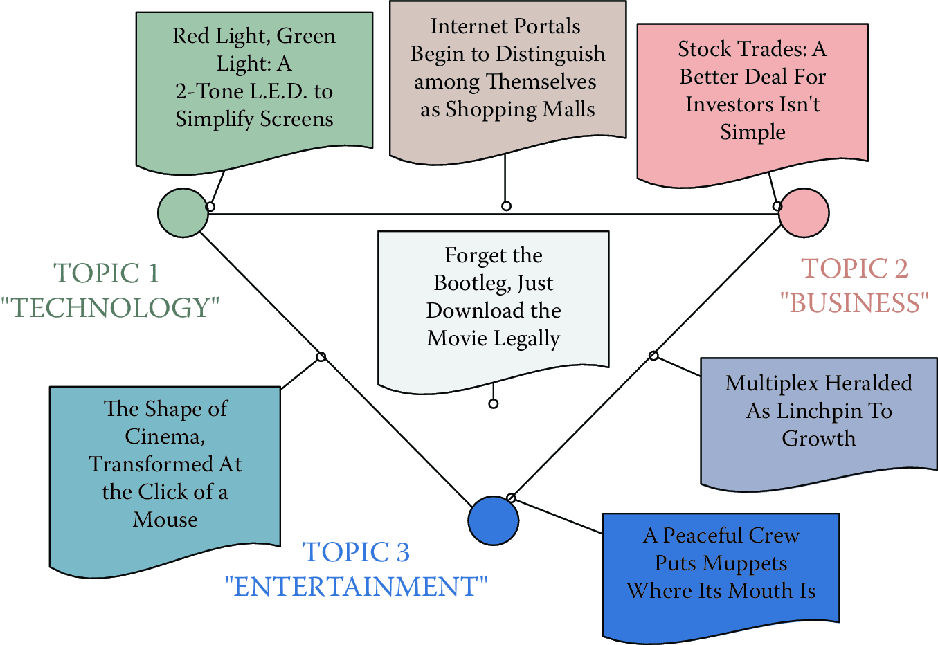
Figure 8.2: Allocations of documents to topics

8.4.5.1 Inferring “topics” from raw text

Algorithmically, the problem can be viewed as: Given a corpus and an integer \(k\) as input, provide the \(k\) topics that best describe the document collection: a process called posterior inference. The most common algorithm for solving this problem is a technique called Gibbs sampling (Geman and Geman 1990).

Gibbs sampling works at the word level to discover the topics that best describe a document collection. Each word is associated with a single topic, explaining why that word appeared in a document. For example, consider the sentence “Hollywood studios are preparing to let people download and buy electronic copies of movies over the Internet.”. Each word in this sentence is associated with a topic: “Hollywood” might be associated with an arts topic; “buy” with a business topic; and “Internet” with a technology topic (Figure 8.3).

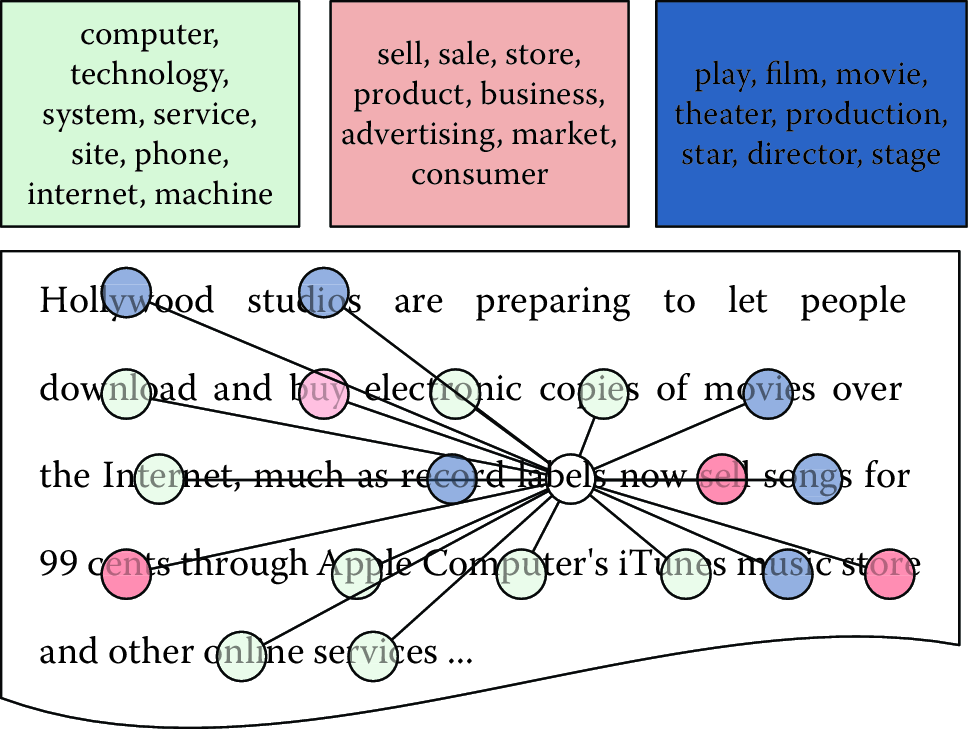
Each word is associated with a topic. Gibbs sampling inference iteratively resamples the topic assignments for each word to discover the most likely topic assignments that explain the document collection

Figure 8.3: Each word is associated with a topic. Gibbs sampling inference iteratively resamples the topic assignments for each word to discover the most likely topic assignments that explain the document collection

This is where we should eventually get. However, we do not know this to start. So, we can initially assign words to topics randomly. This will result in poor topics, but we can make those topics better. We improve these topics by taking each word, pretending that we do not know the topic, and selecting a new topic for the word.

A topic model wants to do two things: it does not want to use many topics in a document, and it does not want to use many words in a topic. So the algorithm will keep track of how many times a document \(d\) has used a topic \(k\), \(N_{d,k}\), and how many times a topic \(k\) has used a word \(w\), \(V_{k,w}\). For notational convenience, it will also be useful to keep track of marginal counts of how many words are in a document, \[N_{d, \cdot} \equiv \sum_k N_{d,k},\] and how many words are associated with a topic, \[V_{k, \cdot} \equiv \sum_w V_{k, w}.\] The algorithm removes the counts for a word from \(N_{d,k}\) and \(V_{k,w}\) and then changes the topic of a word (hopefully to a better topic than the one it had before). Through many thousands of iterations of this process, the algorithm can find topics that are coherent, useful, and characterize the data well.

The two goals of topic modeling—balancing document allocations to topics and topics’ distribution over words—come together in an equation that multiplies them together. A good topic will be both common in a document and explain a word’s appearance well.

Example: Gibbs sampling for topic models

The topic assignment \(z_{d,n}\) of word \(n\) in document \(d\) is proportional to \[p(z_{d,n}=k) \propto \left( \underset{\text{how much doc likes the topic}}{\frac{N_{d,k} + \alpha}{N_{d, \cdot} + K \alpha}} \right) \left(\underset{\text{how much topic likes the word}}{\frac{V_{k,w_{d,n}} + \beta}{V_{k, \cdot} + V \beta}} \right),\] where \(\alpha\) and \(\beta\) are smoothing factors that prevent a topic from having zero probability if a topic does not use a word or a document does not use a topic (Wallach, Mimno, and McCallum 2009). Recall that we do not include the token that we are sampling in the counts for \(N\) or \(V\).

For the sake of concreteness, assume that we have three documents with the following topic assignments:

Document 1: \(^A\)dog\(_3\) \(^B\)cat\(_2\) \(^C\)cat\(_3\) \(^D\)pig\(_1\)
Document 2: \(^E\)hamburger\(_2\) \(^F\)dog\(_3\) \(^G\)hamburger\(_1\)
Document 3: \(^H\)iron\(_1\) \(^I\)iron\(_3\) \(^J\)pig\(_2\) \(^K\)iron\(_2\)

If we want to sample token B (the first instance of of “cat” in document 1), we compute the conditional probability for each of the three topics (\(z=1,2,3\)): \[\begin{aligned} p(z_B = 1) = & \frac{1 + 1.000}{3 + 3.000} \times \frac{0 + 1.000}{3 + 5.000} = 0.333 \times 0.125 = 0.042, \\[4pt] p(z_B = 2) = & \frac{0 + 1.000}{3 + 3.000} \times \frac{0 + 1.000}{3 + 5.000} = 0.167 \times 0.125 = 0.021\mbox{, and} \\[4pt] p(z_B = 3) = & \frac{2 + 1.000}{3 + 3.000} \times \frac{1 + 1.000}{4 + 5.000} = 0.500 \times 0.222 = 0.111.\end{aligned}\] To reiterate, we do not include token B in these counts: in computing these conditional probabilities, we consider topic 2 as never appearing in the document and “cat” as never appearing in topic 2. However, “cat” does appear in topic 3 (token C), so it has a higher probability than the other topics. After renormalizing, our conditional probabilities are \((0.24, 0.12, 0.64)\). We then sample the new assignment of token B to be topic 3 two times out of three. Griffiths and Steyvers (2004) provide more details on the derivation of this equation.

8.4.5.2 Applications of topic models

Topic modeling is most often used for topic exploration, allowing users to understand the contents of large text corpora. Thus, topic models have been used, for example, to understand what the National Institutes of Health funds (Talley et al. 2011); to compare and contrast what was discussed in the North and South in the Civil War (Nelson 2010); and to understand how individuals code in large programming projects (Maskeri, Sarkar, and Heafield 2008).

Topic models can also be used as features to more elaborate algorithms such as machine translation (Hu et al. 2014), detecting objects in images (Wang, Blei, and Fei-Fei 2009), or identifying political polarization (Paul and Girju 2010). Boyd-Graber, Hu, and Mimno (2017) summarize applications of topic models in the humanities, information retrieval, and social sciences.

Blei and McAuliffe (2007) apply topic models to classification and regression tasks such as sentiment analysis. As discussed in the previous chapter, such methods require a feature-based representation of the data. An advantage of using topic models is that the distribution over topics itself can serve as a feature.

For example, to predict whether a legislator will vote on a bill, Gerrish and Blei (2012) learn a topic model that encodes each bill (proposed piece of legislation) as a vector. To predict how a legislator will vote on a bill, the model takes a dot product between the bill’s distribution over topics and a legislator’s ideology vector. The higher score, the more compatible they are and the more likely the legislator is to vote on the bill. Conversely, the lower the score, the less likely it is the legislator will vote on the bill.

This formulation should remind you of logistic regression; however, the features are learned automatically rather than the feature engineering approach described in the last chapter.

Use Case: Document classification

The section above focused on the task of finding topics and themes in a new text data set. In many cases, we already know a set of topics—this could be the set of topics or research fields as described by the Social Science Research Network or the set of sections (local news, international, sports, finance, etc.) in a news publication. The task we often face is to automatically categorize new documents into an existing set of categories. In text analysis, this is called text classification or categorization and uses supervised learning techniques from machine learning described in the earlier chapter.

Text classification typically requires two things: a set of categories we want documents to be categorized into (each document can belong to one or more categories) and a set of documents annotated/tagged with one or more categories from step 1.

For example, if we want to classify Twitter or Facebook posts as being about health or finance, a classification method would take a small number of posts, manually tagged as belonging to either health or finance, and train a classification model. This model can then be used to automatically classify new posts as belonging to either health or finance.

All of the classification (supervised learning) methods we covered in the Machine Learning chapter can be used here once the text data has been processed and converted to a matrix. Neural Networks (Iyyer et al. 2015), Naive Bayes (Lewis 1998), and Support Vector Machines (Zhu et al. 2013) are some of the commonly used methods applied to text data.

Example: Using text to categorize scientific fields

The National Center for Science and Engineering Statistics, the US statistical agency charged with collecting statistics on science and engineering, uses a rule-based system to manually create categories of science; these are then used to categorize research as “physics” or “economics” (Mortensen and Bloch 2005; Organisation of Economic Co-operation and Development 2004). In a rule-based system there is no ready response to the question “how much do we spend on climate change, food safety, or biofuels?” because existing rules have not created such categories. Text analysis techniques can be used to provide such detail without manual collation. For example, data about research awards from public sources and about people funded on research grants from UMETRICS can be linked with data about their subsequent publications and related student dissertations from ProQuest. Both award and dissertation data are text documents that can be used to characterize what research has been done, provide information about which projects are similar within or across institutions, and potentially identify new fields of study (Talley et al. 2011).

Applications

Spam Detection

One simple but ubiquitous example of document classification is spam detection: an email is either an unwanted advertisement (spam) or it is not. Document classification techniques such as naïve Bayes (Lewis 1998) touch essentially every email sent worldwide, making email usable even though most emails are spam.

Sentiment analysis

Instead of being what a document is about, a label \(y\) could also reveal the speaker. A recent subfield of natural language processing is to use machine learning to reveal the internal state of speakers based on what they say about a subject (Pang and Lee 2008). For example, given an example of sentence \(x\), can we determine whether the speaker is a Liberal or a Conservative? Is the speaker happy or sad?

Simple approaches use dictionaries and word counting methods (Pennebaker and Francis 1999), but more nuanced approaches make use of domain-specific information to make better predictions. One uses different approaches to praise a toaster than to praise an air conditioner (Blitzer, Dredze, and Pereira 2007); Liberals and Conservatives each frame health care differently from how they frame energy policy (Nguyen, Boyd-Graber, and Resnik 2013).

Evaluating Text Classification Methods

The metrics used to evaluate text classification methods are the same as those used in supervised learning, as described in the Machine Learning chapter. The most commonly used metrics include accuracy, precision, recall, AUC, and F1 score.

8.5 Word Embeddings and Deep Learning

In discussing topic models, we learned a vector that summarized the content of each document. This is useful for applications where you can use a single, short vector to summarize a document for a downstream machine learning application. However, modern research doesn’t stop there, it learns vector representations of everything from documents down to sentences and words.

First, let’s consider this from a high-level perspective. The goal of representation learning (Bengio, Courville, and Vincent 2013) is to take an input and transform it into a vector that computers can understand. Similar inputs should be close together in vector space. E.g., “dog” and “poodle” should have similar vectors, while “dog” and “chainsaw” should not.

A well-known technique for word representation is word2vec (Mikolov et al. 2013). Using an objective function similar to logistic regression, it predicts, given a word, whether another word will appear in the same context. For example, the dot product for “dog” and “pet”, “dog” and “leash”, and “dog” and “wag” will be high but those for “dog” and “rectitude”, “dog” and “examine”, and “dog” and “cloudy” will be lower. Training a model to do this for all of the words in English will produce vector representations for “dog” and “poodle” that are quite close together.

This model has been well adopted throughout natural language processing (Ward 2017). Downloading word2vec vectors for words and using them as features in your machine learning pipeline (e.g., for document classification by averaging the words in the document) will likely improve a supervised classification task.

But word representations are not the end of the story. A word only makes sense in the context of the sentence in which it appears: e.g., “I deposited my check at the bank” versus “The airplane went into a bank of clouds”. A single word per vector does not capture these subtle effects. More recent models named after Muppets (long, uninteresting story) tries to capture broader relationships between words within sentences to create contextualized representations.

ELMO (Peters et al. 2018) and BERT (Devlin et al. 2019) both use deep learning to take word vectors (a la word2vec) to create representations that make sense given a word’s context. These are also useful features to use in supervised machine learning contexts if higher accuracy is your goal.

However, these techniques are not always the best tools for social scientists. They are not always interpretable—it is often hard to tell why you got the answer you did (Ribeiro, Singh, and Guestrin 2016), and slightly changing the input the models can dramatically change the results (Feng et al. 2018). Given that our goal is often understanding our data, it is probably better to start first with the simpler (and faster methods) mentioned here to understand your data first.

8.6 Text analysis tools

We are fortunate to have access to a set of powerful open source text analysis tools. We describe three here.

The Natural Language Toolkit

The NLTK is a commonly used natural language toolkit that provides a large number of relevant solutions for text analysis. It is Python-based and can be easily integrated into data processing and analytical scripts by a simple import nltk (or similar for any one of its submodules).

The NLTK includes a set of tokenizers, stemmers, lemmatizers and other natural language processing tools typically applied in text analysis and machine learning. For example, a user can extract tokens from a document doc by running the command tokens = nltk.word_tokenize(doc).

Useful text corpora are also present in the NLTK distribution. For example, the stop words list can be retrieved by running the command stops = nltk.corpus.stopwords.words(language). These stop words are available for several languages within NTLK, including English, French, and Spanish.

Similarly, the Brown Corpus or WordNet can be called by running from nltk.corpus import wordnet/brown. After the corpora are loaded, their various properties can be explored and used in text analysis; for example, dogsyn = wordnet.synsets('dog') will return a list of WordNet synsets related to the word “dog.”

Term frequency distribution and \(n\)-gram indexing are other techniques implemented in NLTK. For example, a user can compute frequency distribution of individual terms within a document doc by running a command in Python: fdist = nltk.FreqDist(text). This command returns a dictionary of all tokens with associated frequency within doc.

\(N\)-gram indexing is implemented as a chain-linked collocations algorithm that takes into account the probability of any given two, three, or more words appearing together in the entire corpus. In general, \(n\)-grams can be discovered as easily as running bigrams = nltk.bigrams(text). However, a more sophisticated approach is needed to discover statistically significant word collocations, as we show in Listing Bigrams.

Bird, Klein, and Loper (2009) provide a detailed description of NLTK tools and techniques. See also the official NLTK website.⁶⁸

def bigram_finder(texts):
  # NLTK bigrams from a corpus of documents separated by new line
  tokens_list = nltk.word_tokenize(re.sub("\n"," ",texts))
  bgm    = nltk.collocations.BigramAssocMeasures()
  finder = nltk.collocations.BigramCollocationFinder.from_words(tokens_list)
  scored = finder.score_ngrams( bgm.likelihood_ratio  )

  # Group bigrams by first word in bigram.
  prefix_keys = collections.defaultdict(list)
  for key, scores in scored:
      prefix_keys[key[0]].append((key[1], scores))

  # Sort keyed bigrams by strongest association.
  for key in prefix_keys:
      prefix_keys[key].sort(key = lambda x: -x[1])

Listing: Python code to find bigrams using NLTK

Stanford CoreNLP

While NLTK’s emphasis is on simple reference implementations, Stanford’s CoreNLP (Manning et al. 2014) is focused on fast implementations of cutting-edge algorithms, particularly for syntactic analysis (e.g., determining the subject of a sentence).⁶⁹

MALLET

For probabilistic models of text, MALLET, the MAchine Learning for LanguagE Toolkit (McCallum 2002), often strikes the right balance between usefulness and usability. It is written to be fast and efficient but with enough documentation and easy enough interfaces to be used by novices. It offers fast, popular implementations of conditional random fields (for part-of-speech tagging), text classification, and topic modeling.

Spacy.io

While NLTK is optimized for teaching NLP concepts to students, Spacy.io [http://spacy.io] is optimized for practical application. It is fast, contains many models for well-trodden tasks (classification, parsing, finding entities in sentences, etc.). It also has pre-trained models (including word and sentence representations) that can help practicioners quickly build competitive models.

Pytorch

For the truly adventurous who want to build their own deep learning models for text, PyTorch [http://pytorch.org] offers the flexibility to go from word vectors to complete deep representations of sentences.

8.7 Summary

Many of the new sources of data that are of interest to social scientists is text: tweets, Facebook posts, corporate emails, and the news of the day. However, the meaning of these documents is buried beneath the ambiguities and noisiness of the informal, inconsistent ways by which humans communicate with each other and traditional data analysis methods do not work with text data directly. Despite attempts to formalize the meaning of text data through asking users to tag people, apply metadata, or to create structured representations, these attempts to manually curate meaning are often incomplete, inconsistent, or both.

These aspects make text data difficult to work with, but also a rewarding object of study. Unlocking the meaning of a piece of text helps bring machines closer to human-level intelligence—as language is one of the most quintessentially human activities—and helps overloaded information professionals do their jobs more effectively: understand large corpora, find the right documents, or automate repetitive tasks. And as an added bonus, the better computers become at understanding natural language, the easier it is for information professionals to communicate their needs: one day using computers to grapple with big data may be as natural as sitting down for a conversation over coffee with a knowledgeable, trusted friend.

8.8 Resources

Text analysis is one of the more complex tasks in big data analysis. Because it is unstructured, text (and natural language overall) requires significant processing and cleaning before we can engage in interesting analysis and learning. In this chapter we have referenced several resources that can be helpful in mastering text mining techniques:

The Natural Language Toolkit is one of the most popular Python-based tools for natural language processing. It has a variety of methods and examples that are easily accessible online.⁷⁰ The book by Bird, Klein, and Loper (2009), available online, contains multiple examples and tips on how to use NLTK. This is a great package to use if you want to understand these models.
A paper by Anna Huang (2008) provides a brief overview of the key similarity measures for text document clustering discussed in this chapter, including their strengths and weaknesses in different contexts.
Materials at the MALLET website (McCallum 2002) can be specialized for the unprepared reader but are helpful when looking for specific solutions with topic modeling and machine classification using this toolkit.
We provide an example of how to run topic modeling using MALLET on textual data from the National Science Foundation and Norwegian Research Council award abstracts.⁷¹
If you do not care about understanding and just want models that are easy to use and fast, spaCy [https://spacy.io/] has a useful minimal core of models for the average user. spaCy is the most useful toolkit for the preprocessing steps of dataset preparation.
For more advanced models (classification, tagging, etc.), the AllenNLP toolkit [https://allennlp.org/] is useful if you want to run state of the art models and tweak them just slightly.
Text corpora: A set of multiple similar documents is called a corpus. For
example, the Brown University Standard Corpus of Present-Day American English, or just the Brown Corpus (Francis and Kucera 1979), is a collection of processed documents from works published in the United States in 1961. The Brown Corpus was a historical milestone: it was a machine-readable collection of a million words across 15 balanced genres with each word tagged with its part of speech (e.g., noun, verb, preposition). The British National Corpus (University of Oxford 2006) repeated the same process for British English at a larger scale. The Penn Treebank (Marcus, Santorini, and Marcinkiewicz 1993) provides additional information: in addition to part-of-speech annotation, it provides syntactic annotation. For example, what is the object of the sentence “The man bought the hat”? These standard corpora serve as training data to train the classifiers and machine learning techniques to automatically analyze text (Halevy, Norvig, and Pereira 2009).
The Text Analysis workbook of Chapter Workbooks provides an introduction to topic modeling with Python.⁷²

References

Bengio, Yoshua, Aaron Courville, and Pascal Vincent. 2013. “Representation Learning: A Review and New Perspectives.” IEEE Transactions on Pattern Analysis and Machine Intelligence 35 (8): 1798–1828.

Bird, Steven, Ewan Klein, and Edward Loper. 2009. Natural Language Processing with Python: Analyzing Text with the Natural Language Toolkit. O’Reilly Media.

Blei, David M., and John Lafferty. 2009. “Topic Models.” In Text Mining: Theory and Applications, edited by Ashok Srivastava and Mehran Sahami. Taylor & Francis.

Blei, David M., and Jon D. McAuliffe. 2007. “Supervised Topic Models.” In Advances in Neural Information Processing Systems. MIT Press.

Blei, David M., Andrew Ng, and Michael Jordan. 2003. “Latent Dirichlet Allocation.” Journal of Machine Learning Research 3: 993–1022.

Blitzer, John, Mark Dredze, and Fernando Pereira. 2007. “Biographies, Bollywood, Boom-Boxes and Blenders: Domain Adaptation for Sentiment Classification.” In ACL, 187–205.

Boyd-Graber, Jordan, Yuening Hu, and David Mimno. 2017. Applications of Topic Models. Edited by Doug Oard. Vol. 11. Foundations and Trends in Information Retrieval 2–3. NOW Publishers.

Devlin, Jacob, Ming-Wei Chang, Kenton Lee, and Kristina Toutanova. 2019. “BERT: Pre-Training of Deep Bidirectional Transformers for Language Understanding.” In Conference of the North American Chapter of the Association for Computational Linguistics.

Dunning, Ted. 1993. “Accurate Methods for the Statistics of Surprise and Coincidence.” Computational Linguistics 19 (1). Cambridge, MA: MIT Press: 61–74.

Feng, Shi, Eric Wallace, Alvin Grissom II, Pedro Rodriguez, Mohit Iyyer, and Jordan Boyd-Graber. 2018. “Pathologies of Neural Models Make Interpretation Difficult.” In Empirical Methods in Natural Language Processing. Brussels, Belgium.

Ferragina, Paolo, and Ugo Scaiella. 2010. “TAGME: On-the-Fly Annotation of Short Text Fragments (by Wikipedia Entities).” In Proceedings of the 19th Acm International Conference on Information and Knowledge Management, 1625–8. CIKM 10. New York, NY, USA: Association for Computing Machinery.

Francis, W. Nelson, and Henry Kucera. 1979. “Brown Corpus Manual.” Department of Linguistics, Brown University, Providence, Rhode Island, US.

Geman, Stuart, and Donald Geman. 1990. “Stochastic Relaxation, Gibbs Distributions, and the Bayesian Restoration of Images.” In Readings in Uncertain Reasoning, edited by Glenn Shafer and Judea Pearl, 452–72. Morgan Kaufmann.

Gerrish, Sean M., and David M. Blei. 2012. “The Issue-Adjusted Ideal Point Model.” https://arxiv.org/abs/1209.6004.

Griffiths, Thomas L., and Mark Steyvers. 2004. “Finding Scientific Topics.” Proceedings of the National Academy of Sciences 101 (Suppl. 1): 5228–35.

Halevy, Alon, Peter Norvig, and Fernando Pereira. 2009. “The Unreasonable Effectiveness of Data.” IEEE Intelligent Systems 24 (2). Piscataway, NJ: IEEE Educational Activities Department: 8–12.

Hofmann, Thomas. 1999. “Probabilistic Latent Semantic Analysis.” In Proceedings of Uncertainty in Artificial Intelligence.

Hu, Yuening, Ke Zhai, Vlad Eidelman, and Jordan Boyd-Graber. 2014. “Polylingual Tree-Based Topic Models for Translation Domain Adaptation.” In Proceedings of the 52nd Annual Meeting of the Association for Computational Linguistics. Baltimore, MD.

Huang, Anna. 2008. “Similarity Measures for Text Document Clustering.” Paper presented at New Zealand Computer Science Research Student Conference, Christchurch, New Zealand, April 14–18.

Iyyer, Mohit, Varun Manjunatha, Jordan Boyd-Graber, and Hal Daumé III. 2015. “Deep Unordered Composition Rivals Syntactic Methods for Text Classification.” In Association for Computational Linguistics.

Kiss, Tibor, and Jan Strunk. 2006. “Unsupervised Multilingual Sentence Boundary Detection.” Computational Linguistics 32 (4). Cambridge, MA: MIT Press: 485–525.

Kong, Lingpeng, Nathan Schneider, Swabha Swayamdipta, Archna Bhatia, Chris Dyer, and Noah A. Smith. 2014. “A Dependency Parser for Tweets.” In Proceedings of the 2014 Conference on Empirical Methods in Natural Language Processing (EMNLP), 1001–12. Association for Computational Linguistics.

Kullback, Solomon, and Richard A. Leibler. 1951. “On Information and Sufficiency.” Annals of Mathematical Statistics 22 (1). JSTOR: 79–86.

Lafferty, John D., Andrew McCallum, and Fernando C. N. Pereira. 2001. “Conditional Random Fields: Probabilistic Models for Segmenting and Labeling Sequence Data.” In Proceedings of the Eighteenth International Conference on Machine Learning, 282–89. Morgan Kaufmann.

Landauer, Thomas, and Susan Dumais. 1997. “Solutions to Plato’s Problem: The Latent Semantic Analysis Theory of Acquisition, Induction and Representation of Knowledge.” Psychological Review 104 (2): 211–40.

Lewis, David D. 1998. “Naive (Bayes) at Forty: The Independence Assumption in Information Retrieval.” In Proceedings of European Conference of Machine Learning, 4–15.

Malmkjær, K. 2002. The Linguistics Encyclopedia. Routledge.

Manning, Christopher D., Mihai Surdeanu, John Bauer, Jenny Finkel, Steven J. Bethard, and David McClosky. 2014. “The Stanford CoreNLP Natural Language Processing Toolkit.” In Proceedings of 52nd Annual Meeting of the Association for Computational Linguistics: System Demonstrations, 55–60.

Marcus, Mitchell P., Beatrice Santorini, and Mary A. Marcinkiewicz. 1993. “Building a Large Annotated Corpus of English: The Penn Treebank.” Computational Linguistics 19 (2): 313–30.

Maskeri, Girish, Santonu Sarkar, and Kenneth Heafield. 2008. “Mining Business Topics in Source Code Using Latent Dirichlet Allocation.” In Proceedings of the 1st India Software Engineering Conference, 113–20. ACM.

McCallum, Andrew Kachites. 2002. “MALLET: A Machine Learning for Language Toolkit.” http://mallet.cs.umass.edu.

Meij, Edgar, Marc Bron, Laura Hollink, Bouke Huurnink, and Maarten Rijke. 2009. “Learning Semantic Query Suggestions.” In Proceedings of the 8th International Semantic Web Conference, 424–40. ISWC ’09. Springer.

Mikolov, Tomas, Ilya Sutskever, Kai Chen, Greg S. Corrado, and Jeff Dean. 2013. “Distributed Representations of Words and Phrases and Their Compositionality.” In Advances in Neural Information Processing Systems, 3111–9. Morgan Kaufmann.

Molina, Giovanni, Fahad AlGhamdi, Mahmoud Ghoneim, Abdelati Hawwari, Nicolas Rey-Villamizar, Mona Diab, and Thamar Solorio. 2016. “Overview for the Second Shared Task on Language Identification in Code-Switched Data.” In Proceedings of the Second Workshop on Computational Approaches to Code Switching, 40–49. Austin, Texas: Association for Computational Linguistics.

Mortensen, Peter Stendahl, and Carter Walter Bloch. 2005. Oslo Manual: Guidelines for Collecting and Interpreting Innovation Data. Organisation for Economic Co-operation and Development.

Navigli, Roberto, Stefano Faralli, Aitor Soroa, Oier de Lacalle, and Eneko Agirre. 2011. “Two Birds with One Stone: Learning Semantic Models for Text Categorization and Word Sense Disambiguation.” In Proceedings of the 20th Acm International Conference on Information and Knowledge Management. ACM.

Nelson, Robert K. 2010. “Mining the Dispatch.” http://dsl.richmond.edu/dispatch/.

Nguyen, Viet-An, Jordan Boyd-Graber, and Philip Resnik. 2012. “SITS: A Hierarchical Nonparametric Model Using Speaker Identity for Topic Segmentation in Multiparty Conversations.” In Proceedings of the Association for Computational Linguistics. Jeju, South Korea.

Nguyen, Viet-An, Jordan Boyd-Graber, and Philip Resnik. 2013. “Lexical and Hierarchical Topic Regression.” In Advances in Neural Information Processing Systems. Lake Tahoe, Nevada.

Nguyen, Viet-An, Jordan Boyd-Graber, Philip Resnik, and Jonathan Chang. 2014. “Learning a Concept Hierarchy from Multi-Labeled Documents.” In Proceedings of the Annual Conference on Neural Information Processing Systems. Morgan Kaufmann.

Nguyen, Viet-An, Jordan Boyd-Graber, Philip Resnik, and Kristina Miler. 2015. “Tea Party in the House: A Hierarchical Ideal Point Topic Model and Its Application to Republican Legislators in the 112th Congress.” In Association for Computational Linguistics. Beijing, China.

Niculae, Vlad, Srijan Kumar, Jordan Boyd-Graber, and Cristian Danescu-Niculescu-Mizil. 2015. “Linguistic Harbingers of Betrayal: A Case Study on an Online Strategy Game.” In Association for Computational Linguistics. Beijing, China.

Organisation of Economic Co-operation and Development. 2004. “A Summary of the Frascati Manual.” Main Definitions and Conventions for the Measurement of Research and Experimental Development 84.

Ott, Myle, Yejin Choi, Claire Cardie, and Jeffrey T. Hancock. 2011. “Finding Deceptive Opinion Spam by Any Stretch of the Imagination.” In Proceedings of the 49th Annual Meeting of the Association for Computational Linguistics: Human Language Technologies—Volume 1, 309–19. HLT ’11. Stroudsburg, PA: Association for Computational Linguistics.

Pang, Bo, and Lillian Lee. 2008. Opinion Mining and Sentiment Analysis. Paperback; Now Publishers.

Paul, Michael, and Roxana Girju. 2010. “A Two-Dimensional Topic-Aspect Model for Discovering Multi-Faceted Topics.” In Association for the Advancement of Artificial Intelligence.

Pennebaker, James W., and Martha E. Francis. 1999. Linguistic Inquiry and Word Count. Loose Leaf; Lawrence Erlbaum.

Peters, Matthew, Mark Neumann, Mohit Iyyer, Matt Gardner, Christopher Clark, Kenton Lee, and Luke Zettlemoyer. 2018. “Deep Contextualized Word Representations.” In Conference of the North American Chapter of the Association for Computational Linguistics.

Plank, Barbara, Anders Søgaard, and Yoav Goldberg. 2016. “Multilingual Part-of-Speech Tagging with Bidirectional Long Short-Term Memory Models and Auxiliary Loss.” In Proceedings of the 54th Annual Meeting of the Association for Computational Linguistics (Volume 2: Short Papers), 412–18. Berlin, Germany: Association for Computational Linguistics.

Rabiner, Lawrence R. 1989. “A Tutorial on Hidden Markov Models and Selected Applications in Speech Recognition.” Proceedings of the IEEE 77 (2): 257–86.

Ramage, Daniel, David Hall, Ramesh Nallapati, and Christopher Manning. 2009. “Labeled LDA: A Supervised Topic Model for Credit Attribution in Multi-Labeled Corpora.” In Proceedings of Empirical Methods in Natural Language Processing.

Ribeiro, Marco Tulio, Sameer Singh, and Carlos Guestrin. 2016. “‘Why Should I Trust You?’: Explaining the Predictions of Any Classifier.” In Proceedings of the 22nd ACM SIGKDD International Conference on Knowledge Discovery and Data Mining, 1135–44. San Francisco, CA, USA.

Ritter, Alan, Mausam, Oren Etzioni, and Sam Clark. 2012. “Open Domain Event Extraction from Twitter.” In Proceedings of the 18th Acm Sigkdd International Conference on Knowledge Discovery and Data Mining, 1104–12. KDD 12. New York, NY, USA: Association for Computing Machinery.

Salton, Gerard. 1968. Automatic Information Organization and Retrieval. McGraw-Hill.

Sandhaus, Evan. 2008. “The New York Times Annotated Corpus.” Philadelphia: Linguistic Data Consortium, http://www.ldc.upenn.edu/Catalog/CatalogEntry.jsp? catalogId=LDC2008T19.

Talley, Edmund M., David Newman, David Mimno, Bruce W. Herr, Hanna M. Wallach, Gully A. P. C. Burns, A. G. Miriam Leenders, and Andrew McCallum. 2011. “Database of NIH Grants Using Machine-Learned Categories and Graphical Clustering.” Nature Methods 8 (6): 443–44.

Tuarob, Suppawong, Line C. Pouchard, and C. Lee Giles. 2013. “Automatic Tag Recommendation for Metadata Annotation Using Probabilistic Topic Modeling.” In Proceedings of the 13th ACM/IEEE-CS Joint Conference on Digital Libraries, 239–48. JCDL ’13. ACM.

University of Oxford. 2006. “British National Corpus.” http://www.natcorp.ox.ac.uk/.

Wallach, Hanna, David Mimno, and Andrew McCallum. 2009. “Rethinking LDA: Why Priors Matter.” In Advances in Neural Information Processing Systems.

Wang, Chong, David Blei, and Li Fei-Fei. 2009. “Simultaneous Image Classification and Annotation.” In Computer Vision and Pattern Recognition.

Wang, Yi, Hongjie Bai, Matt Stanton, Wen-Yen Chen, and Edward Y. Chang. 2009. “PLDA: Parallel Latent Dirichlet Allocation for Large-Scale Applications.” In International Conference on Algorithmic Aspects in Information and Management.

Ward, Kenneth Church. 2017. “Word2Vec.” Natural Language Engineering 23 (1). Cambridge University Press: 155–62.

Yates, Dave, and Scott Paquette. 2010. “Emergency Knowledge Management and Social Media Technologies: A Case Study of the 2010 Haitian Earthquake.” In Proceedings of the 73rd Asis&T Annual Meeting on Navigating Streams in an Information Ecosystem. Vol. 47. ASIS&T ’10. Silver Springs, MD: American Society for Information Science.

Zeng, Qing T., Doug Redd, Thomas C. Rindflesch, and Jonathan R. Nebeker. 2012. “Synonym, Topic Model and Predicate-Based Query Expansion for Retrieving Clinical Documents.” In American Medical Informatics Association Annual Symposium, 1050–9.

Zhu, Jun, Ning Chen, Hugh Perkins, and Bo Zhang. 2013. “Gibbs Max-Margin Topic Models with Fast Sampling Algorithms.” In Proceedings of the International Conference of Machine Learning.

This is often the term used but is a fallacy. There is a lot of structure in text—the structure of chapters, paragraphs, sentences, and syntax (Marcus, Santorini, and Marcinkiewicz 1993) within a sentence allows you, the reader, to understand what we’re writing here. Nevertheless you will see the term unstructured data often used to refer to text or in some cases to other forms of non tabular data such as images and videos↩
See Chapter Machine Learning for a discussion of speech recognition, which can turn spoken language into text↩
If you have examples from your own research using the methods we describe in this chapter, please submit a link to the paper (and/or code) here: https://textbook.coleridgeinitiative.org/submitexamples ↩
Cleaning and processing are discussed extensively in Chapter Record Linkage.↩
Term weighting is an example of feature engineering discussed in Chapter Machine Learning.↩
http://www.nltk.org ↩
https://stanfordnlp.github.io/CoreNLP/↩
http://www.nltk.org ↩
http://www.umiacs.umd.edu/~jbg/lda_demo ↩
See https://workbooks.coleridgeinitiative.org.↩