Chapter 7 Machine Learning
Rayid Ghani and Malte Schierholz
This chapter introduces you to the use of machine learning in tackling social science and public policy problems. We cover the end-to-end machine learning process and focus on clustering and classification methods. After reading this chapter, you should have an overview of the components of a machine learning pipeline and methods, and know how to use those in solving social science problems. We have written this chapter to give an intuitive explanation for the methods and to provide a framework and practical tips on how to use them in practice.
7.1 Introduction
You have probably heard of “machine learning” but are not sure exactly what it is, how it differs from traditional statistics, and what you, as social scientists, can do with it. In this chapter, we will demystify machine learning, draw connections to what you already know from statistics and data analysis, and go deeper into some of the novel concepts and methods that have been developed in this field. Although the field originates from computer science, it has been influenced quite heavily by math and statistics in the past 15–20 years. As you will see, many of the concepts you will learn are not entirely new, but are simply called something else. For example, you already are familiar with logistic regression (a classification method that falls under the supervised learning framework in machine learning) and cluster analysis (a form of unsupervised learning). You will also learn about new methods that are more exclusively used in machine learning, such as random forests, support vector machines, and neural networks. We will keep formalisms to a minimum and focus on getting the intuition across, as well as providing practical tips. Our hope is this chapter will make you comfortable and familiar with machine learning vocabulary, concepts, and processes, and allows you to further explore and use these methods and tools in your own research and practice.
7.2 What is machine learning?
When humans improve their skills with experience, they are said to learn. Is it also possible to program computers to do the same? Arthur Samuel, who coined the term machine learning in 1959 (Samuel 1959), was a pioneer in this area, programming a computer to play checkers. The computer played against itself and human opponents, improving its performance with every game. Eventually, after sufficient training (and experience), the computer became a better player than the human programmer. Today, machine learning has grown significantly beyond learning to play checkers. Machine learning systems have learned to drive (and park) autonomous cars, are embedded inside robots, can recommend books, products, and movies we are (sometimes) interested in, identify drugs, proteins, and genes that should be investigated further to cure diseases, detect cancer and other pathologies in x-rays and other types of medical imaging, help us understand how the human brain learns language, help identify which voters are persuadable in elections, detect which students are likely to need extra support to graduate high school on time, and help solve many more problems. Over the past 20 years, machine learning has become an interdisciplinary field spanning computer science, artificial intelligence, databases, and statistics. At its core, machine learning seeks to design computer systems that improve over time with more experience. In one of the earlier books on machine learning, Tom Mitchell gives a more operational definition, stating that: “A computer program is said to learn from experience \(E\) with respect to some class of tasks \(T\) and performance measure \(P\), if its performance at tasks in \(T\), as measured by \(P\), improves with experience \(E\)” (Mitchell 1997). We like this definition because it is task-focused and allows us to think of machine learning as a tool used inside a larger system to improve outcomes that we care about.
Box: Commercial machine learning examples
Speech recognition: Speech recognition software uses machine learning algorithms that are built on large amounts of initial training data. Machine learning allows these systems to be tuned and adapt to individual variations in speaking as well as across different domains.
Autonomous cars: The ongoing development of self-driving cars applies techniques from machine learning. An onboard computer continuously analyzes the incoming video and sensor streams in order to monitor the surroundings. Incoming data are matched with annotated images to recognize objects like pedestrians, traffic lights, and potholes. In order to assess the different objects, huge training data sets are required where similar objects already have been identified. This allows the autonomous car to decide on which actions to take next.
Fraud detection: Many public and private organizations face the problem of fraud and abuse. Machine learning systems are widely used to take historical cases of fraud and flag fraudulent transactions as they take place. These systems have the benefit of being adaptive, and improving with more data over time.
Personalized ads: Many online stores have personalized recommendations promoting possible products of interest. Based on individual shopping history and what other similar users bought in the past, the website predicts products a user may like and tailors recommendations. Netflix and Amazon are two examples of companies whose recommendation software predicts how a customer would rate a certain movie or product and then suggests items with the highest predicted ratings. Of course there are some caveats here, since they then adjust the recommendations to maximize profits.
Face recognition: Surveillance systems, social networking platforms, and imaging software all use face detection and face recognition to first detect faces in images (or video) and then tag them with individuals for various tasks. These systems are trained by giving examples of faces to a machine learning system which then learns to detect new faces, and tag known individuals. The bias and fairness chapter will highlight some concerns with these types of systems.
Box: Social Science machine learning examples
Potash et al (2015) worked with the Chicago Department of Public Health and used random forests (a machine learning classification method) to predict which children are at risk of lead poisoning. This early warning system was then used to prioritize lead hazard inspections to detect and remediate lead hazards before they had an adverse effect on the child.
Carton et al (2016) used a collection of machine learning methods to identify police officers at risk of adverse behavior, such as unjustified use of force or unjustified shootings or sustained complaints, to prioritize preventive interventions such as training and counseling.
Athey and Wager (2019) use a modification of random forests to estimate heterogeneous treatment effects using a data set from The National Study of Learning Mindsets to evaluate the impact of interventions to improve student achievement.
Voigt et al (2017) uses machine learning methods to analyze footage from body-worn cameras and understand the respectfulness of police officer language toward white and black community members during routine traffic stops.
Machine learning grew from the need for systems that were adaptive, scalable, and cost-effective to build and maintain. A lot of tasks now being done using machine learning used to be done by rule-based systems, where experts would spend considerable time and effort developing and maintaining the rules. The problem with those systems was that they were rigid, not adaptive, hard to scale, and expensive to maintain. Machine learning systems started becoming popular because they could improve the system along all of these dimensions49. Box Applications mentions several examples where machine learning is being used in commercial applications today. Social scientists are uniquely placed today to take advantage of the same advances in machine learning by having better methods to solve several key problems they are tackling. Box Social Science describes a few social science and policy problems that are being tackled using machine learning today.50
This chapter is not an exhaustive introduction to machine learning. There are many books that have done an excellent job of that (Flach 2012; Hastie, Tibshirani, and Friedman 2001; Mitchell 1997). Instead, we present a short and accessible introduction to machine learning for social scientists, give an overview of the overall machine learning process, provide an intuitive introduction to machine learning methods, give some practical tips that will be helpful in using these methods, and leave a lot of the statistical theory to machine learning textbooks. As you read more about machine learning in the research literature or the media, you will encounter names of other fields that are related (and practically the same for most social science audiences), such as statistical learning, data mining, and pattern recognition.
7.3 Types of analysis
A lot of the data analysis tasks that social scientists do can be broken down into four types:
Description: The goal is to describe patterns or groupings in historical data. You’re already familiar with descriptive statistics and exploratory data analysis methods, and we will cover more advanced versions of those later in this chapter under Unsupervised Learning.
Detection: The goal here is not to necessarily understand historical behavior but to detect new or emerging anomalies, events, or patterns as they happen. A typical example is early outbreak detection for infectious diseases in order to inform public health officials.
Prediction: The goal here is to use the same historical data as the description and detection methods, but use it to predict events and behaviors in the future.
Behavior Change (or Causal Inference): The goal here is to understand the causal relationships in the data in order to influence the outcomes we care about.
In this chapter, we will mostly focus on Description and Prediction methods but there is a lot of work going in developing and using machine learning methods for detection as well as for behavior change and causal inference.
7.4 The Machine Learning process
When solving problems using machine learning methods, it is important to think of the larger data-driven problem-solving process of which these methods are a small part51. A typical machine learning problem requires researchers and practitioners to take the following steps:
Understand the problem and goal: This sounds obvious but is often nontrivial. Problems typically start as vague descriptions of a goal—improving health outcomes, increasing graduation rates, understanding the effect of a variable \(X\) on an outcome \(Y\), etc. It is really important to work with people who understand the domain being studied to discuss and define the problem more concretely. What is the analytical formulation of the metric that you are trying to improve? The Data Science Project Scoping Guide52 is a good place to start when doing problem scoping for social science or policy problems
Formulate it as a machine learning problem: Is it a classification problem or a regression problem? Is the goal to build a model that generates a ranked list prioritized by risk of an outcome, or is it to detect anomalies as new data come in? Knowing what kinds of tasks machine learning can solve will allow you to map the problem you are working on to one or more machine learning settings and give you access to a suite of methods appropriate for that task.
Data exploration and preparation: Next, you need to carefully explore the data you have. What additional data do you need or have access to? What variable will you use to match records for integrating different data sources? What variables exist in the data set? Are they continuous or categorical? What about missing values? Can you use the variables in their original form or do you need to alter them in some way?
Feature engineering: In machine learning language, what you might know as independent variables or predictors or factors or covariates are called “features.” Creating good features is probably the most important step in the machine learning process. This involves doing transformations, creating interaction terms, or aggregating over data points or over time and space.
Modeling: Having formulated the problem and created your features, you now have a suite of methods to choose from. It would be great if there were a single method that always worked best for a specific type of problem, but that would make things too easy. Each method makes a difference assumption about the structure and distribution of the data and with large amounts of high-dimensional data53, it is difficult to know apriori which assumption will best match the data we have. Typically, in machine learning, you take a collection of methods and try them out to empirically validate which one works the best for your problem. This process not only helps you select the best method for your problem but also helps you understand the structure of your data. We will give an overview of leading methods that are being used today in this chapter.
Model Interpretation: Once we have built the machine learning models, we also want to understand what they are, which predictors they found important, and how much, what types of entities they flagged as high risk (and why), where they made errors, etc. All of these fall under the model interpretation, interpretability, explainability umbrella which is an active area of research right now in machine learning.
Model Selection: As you build a large number of possible models, you need a way to select the model that is the “best”. This part of the chapter will cover methodology to first test the models on historical data as well as discuss a variety of evaluation metrics. While this chapter will focus mostly on traditionally used metrics, Chapter Bias and Fairness will expand on this using bias and fairness related metrics. It is important to note that sometimes the machine learning literature will call this step the “validation” step using historical data, but we want to distinguish it here from validation, which is the next step.
Model Validation: The next step, after model selection (using historical data) is validation. Validate on new data, as well as designing and running field trials or experiments.
Deployment and Monitoring: Once you have selected the best model and validated it using historical data as well as a field trial, you are ready to put the model into practice. You still have to keep in mind that new data will be coming in, the world will be changing, and the model might also (need to) change over time. We will not cover too much of those aspects in this chapter, but they are important to keep in mind when putting the machine learning work in to practice.
Although each step in this process is critical, a thorough description of each is out of scope. This chapter will focus on models, terms, and techniques that form the core of machine learning.
7.5 Problem formulation: Mapping a problem to machine learning methods
When working on a new problem, one of the first things we need to do is to map it to a class of machine learning methods. In general, the problems we will tackle, including the examples above, can be grouped into two major categories:
Supervised learning: These are problems where there exists a target variable (continuous or discrete) that we want to predict or classify data into. Classification, prediction, and regression all fall into this category. More formally, supervised learning methods predict a value \(Y\) given input(s) \(X\) by learning (or estimating or fitting or training) a function \(F\), where \(F(X) = Y\). Here, \(X\) is the set of variables (known as features in machine learning, or in other fields as predictors) provided as input and \(Y\) is the target/dependent variable or a label (as it is known in machine learning).
The goal of supervised learning methods is to search for that function \(F\) that best estimates or predicts \(Y\). When the output \(Y\) is categorical, this is known as classification. When \(Y\) is a continuous value, this is called regression. Sound familiar?
One key distinction in machine learning is that the goal is not just to find the best function \(F\) that can estimate or predict \(Y\) for observed outcomes (known \(Y\)s) but to find one that best generalizes to new, unseen data, often in the future. This distinction makes methods more focused on generalization and less on just fitting the data we have as best as we can. It is important to note that you do that implicitly when performing regression by not adding more and more higher-order terms to get better fit statistics. By getting better fit statistics, we overfit to the data and the performance on new (unseen) data often goes down. Methods like the lasso (Tibshirani 1996) penalize the model for having too many terms by performing what is known as regularization54.
Unsupervised learning: These are problems where there does not exist a target variable that we want to predict but we want to understand “natural” groupings or patterns in the data. Clustering is the most common example of this type of analysis where you are given \(X\) and want to group similar \(X\)s together. You may have heard of “segmentation” that’s used in the marketing world to group similar customers together using clustering techniques. Principal components analysis (PCA) and related methods also fall into the unsupervised learning category.
In between the two extremes of supervised and unsupervised learning, there is a spectrum of methods that have different levels of supervision involved (Figure 7.1). Supervision in this case is the presence of target variables (known in machine learning as labels). In unsupervised learning, none of the data points have labels. In supervised learning, all data points have labels. In between, either the percentage of examples with labels can vary or the types of labels can vary. We do not cover the weakly supervised and semi-supervised methods much in this chapter, but this is an active area of research in machine learning. Zhu (2008) provides more details.
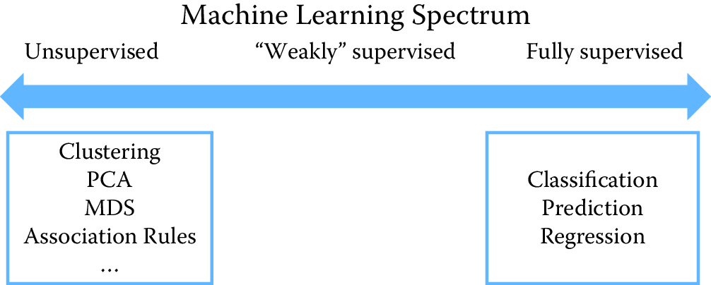
Figure 7.1: Spectrum of machine learning methods from unsupervised to supervised learning
7.5.1 Features
Before we get to models and methods, we need to turn our raw data into “features”. In social science, they are not called features but instead are known as variables or predictors (or covariates if you’re doing regression).55 Feature generation (or engineering, as it is often called) is where a large chunk of the time is spent in the machine learning process. This is also the phase where previous research and learnings from the domain being tackled can be incorporated into the machine learning process. As social science researchers or practitioners, you have spent a lot of time constructing features, using transformations, dummy variables, and interaction terms. All of that is still required and critical in the machine learning framework. One difference you will need to get comfortable with is that instead of carefully selecting a few predictors, machine learning systems tend to encourage the creation of lots of features and then empirically use holdout data to perform regularization and model selection. It is common to have models that are trained on thousands of features. Of course, it is important to keep in mind that increasing the number of features requires you to have enough data so that you’re not overfitting. Commonly used approaches to create features include:
Transformations, such as log, square, and square root.
Dummy (binary) variables: This is often done by taking categorical variables (such as city) and creating a binary variable for each value (one variable for each city in the data). These are also called indicator variables.
Discretization: Several methods require features to be discrete instead of continuous. Several approaches exist to convert continuous variables into discrete ones, the most common of which is equal-width binning.
Aggregation: Aggregate features often constitute the majority of features for a given problem. These aggregations use different aggregation functions (count, min, max, average, standard deviation, etc.), often over varying windows of time and space. For example, given urban data, we would want to calculate the number (and min, max, mean, variance) of crimes within an \(m\)-mile radius of an address in the past \(t\) months for varying values of \(m\) and \(t\), and then to use all of them as features in a classification problem. Spatiotemporal aggregation features are going to be extremely important as you build machine learning models.
In general, it is a good idea to have the complexity in features and use a simple model, rather than using more complex models with simple features. Keeping the model simple makes it faster to train and easier to understand and explain.
7.6 Methods
We will start by describing unsupervised learning methods and then go on to supervised learning methods. We focus here on the intuition behind the methods and the algorithm, as well as some practical tips, rather than on the statistical theory that underlies the methods. We encourage readers to refer to machine learning books listed in Section Resources. Box Vocabulary gives brief definitions of several terms we will use in this section.
Box: Machine learning vocabulary
Learning: In machine learning, you will notice the term learning that will be used in the context of “learning” a model. This is what you probably know as fitting or estimating a function, or training or building a model. These terms are all synonyms and are used interchangeably in the machine learning literature.
Examples: These are data points, rows, observations, or instances.
Features: These are independent variables, attributes, predictor variables, and explanatory variables.
Labels: These include the response variable, dependent variable, target variable, or outcomes.
Underfitting: This happens when a model is too simple and does not capture the structure of the data well enough.
Overfitting: This happens when a model is possibly too complex and models the noise in the data, which can result in poor generalization performance. Using in-sample measures to do model selection can result in that.
Regularization: This is a general method to avoid overfitting by applying additional constraints to the model that is learned. For example, in building logistic regression models, a common approach is to make sure the model weights (coefficients) are, on average, small in magnitude. Two common regularizations are \(L_1\) regularization (used by the lasso), which has a penalty term that encourages the sum of the absolute values of the parameters to be small; and \(L_2\) regularization, which encourages the sum of the squares of the parameters to be small.
7.6.1 Unsupervised learning methods
As mentioned earlier, unsupervised learning methods are used when we do not have a target variable to estimate or predict but want to understand clusters, groups, or patterns in the data. These methods are often used for data exploration, as in the following examples:
When faced with a large corpus of text data—for example, email records, congressional bills, speeches, or open-ended free-text survey responses—unsupervised learning methods are often used to understand and get a handle on the patterns in our data.
Given a data set about students and their behavior over time (academic performance, grades, test scores, attendance, etc.), one might want to understand typical behaviors as well as trajectories of these behaviors over time. Unsupervised learning methods (clustering) can be applied to these data to get student “segments” with similar behavior.
Given a data set about publications or patents in different fields, we can use unsupervised learning methods (association rules) to figure out which disciplines have the most collaboration and which fields have researchers who tend to publish across different fields.
Given a set of people who are at high risk of recidivism, clustering can be used to understand different groups of people within the high risk set, to determine intervention programs that may need to be created.
Clustering
Clustering is the most common unsupervised learning technique and is used to group data points together that are similar to each other. The goal of clustering methods is to produce with high intra-cluster (within) similarity and low inter-cluster (between) similarity.
Clustering algorithms typically require a distance (or similarity) metric56 to generate clusters. They take a data set and a distance metric (and sometimes additional parameters), and they generate clusters based on that distance metric. The most common distance metric used is Euclidean distance, but other commonly used metrics are Manhattan, Minkowski, Chebyshev, cosine, Hamming, Pearson, and Mahalanobis. Often, domain-specific similarity metrics can be designed for use in specific problems. For example, when performing the record linkage tasks discussed in Chapter Record Linkage, you can design a similarity metric that compares two first names and assigns them a high similarity (low distance) if they both map to the same canonical name, so that, for example, Sammy and Sam map to Samuel.
Most clustering algorithms also require the user to specify the number of clusters (or some other parameter that indirectly determines the number of clusters) in advance as a parameter. This is often difficult to do a priori and typically makes clustering an iterative and interactive task. Another aspect of clustering that makes it interactive is often the difficulty in automatically evaluating the quality of the clusters. While various analytical clustering metrics have been developed, the best clustering is task-dependent and thus must be evaluated by the user. There may be different clusterings that can be generated with the same data. You can imagine clustering similar news stories based on the topic content, based on the writing style or based on sentiment. The right set of clusters depends on the user and the task they have. Clustering is therefore typically used for exploring the data, generating clusters, exploring the clusters, and then rerunning the clustering method with different parameters or modifying the clusters (by splitting or merging the previous set of clusters). Interpreting a cluster can be nontrivial: you can look at the centroid of a cluster, look at frequency distributions of different features (and compare them to the prior distribution of each feature), or you can build a decision tree (a supervised learning method we will cover later in this chapter) where the target variable is the cluster ID that can describe the cluster using the features in your data. A good example of a tool that allows interactive clustering from text data is Ontogen (Fortuna, Grobelnik, and Mladenic 2007).
\(k\)-means clustering
The most commonly used clustering algorithm is called \(k\)-means, where \(k\) defines the number of clusters. The algorithm works as follows:
Select \(k\) (the number of clusters you want to generate).
Initialize by selecting \(k\) points as centroids of the \(k\) clusters. This is typically done by selecting \(k\) points uniformly at random.
Assign each point a cluster according to the nearest centroid.
Recalculate cluster centroids based on the assignment in (3) as the mean of all data points belonging to that cluster.
Repeat (3) and (4) until convergence.
The algorithm stops when the assignments do not change from one iteration to the next (Figure 7.2). The final set of clusters, however, depend on the starting points. If they are initialized differently, it is possible that different clusters are obtained. One common practical trick is to run \(k\)-means several times, each with different (random) starting points. The \(k\)-means algorithm is fast, simple, and easy to use, and is often a good first clustering algorithm to try and see if it fits your needs. When the data are of the form where the mean of the data points cannot be computed, a related method called \(K\)-medoids can be used (Park and Jun 2009).
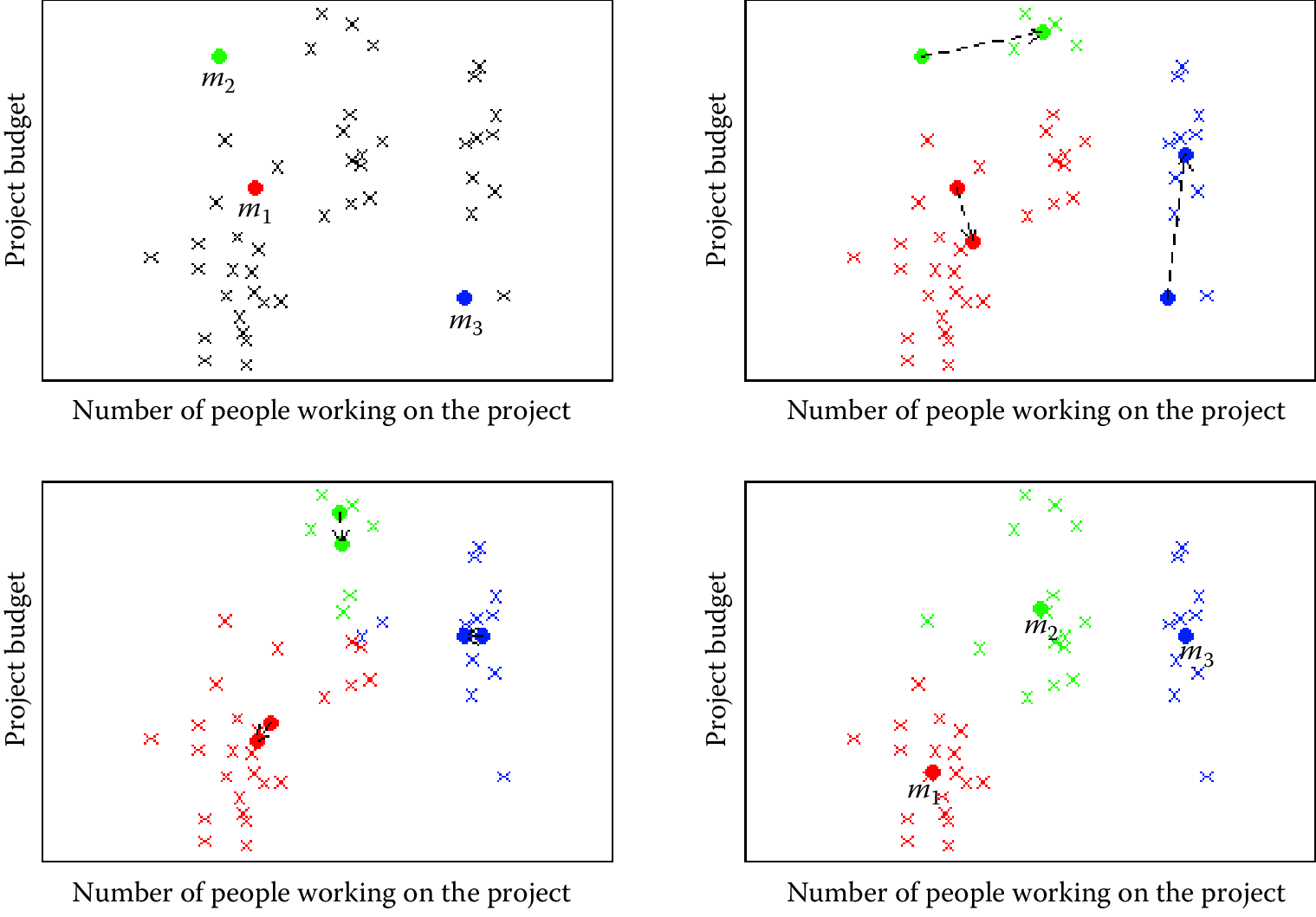
Figure 7.2: Example of \(k\)-means clustering with \(k = 3\). The upper left panel shows the distribution of the data and the three starting points \(m_1\), \(m_2\), \(m_3\) placed at random. On the upper right we see what happens in the first iteration. The cluster means move to more central positions in their respective clusters. The lower left panel shows the second iteration. After six iterations the cluster means have converged to their final destinations and the result is shown in the lower right panel
Expectation-maximization (EM) clustering
You may be familiar with the EM algorithm in the context of imputing missing data. EM is a general approach to maximum likelihood in the presence of incomplete data. However, it is also used as a clustering method where the missing data are the clusters a data point belongs to. Unlike \(k\)-means, where each data point gets assigned to only one cluster, EM does a soft assignment where each data point gets a probabilistic assignment to various clusters. The EM algorithm iterates until the estimates converge to some (locally) optimal solution.
The EM algorithm is fairly good at dealing with outliers as well as high-dimensional data, compared to \(k\)-means. It also has a few limitations. First, it does not work well with a large number of clusters or when a cluster contains few examples. Also, when the value of \(k\) is larger than the number of actual clusters in the data, EM may not give reasonable results.
Mean shift clustering
Mean shift clustering works by finding dense regions in the data by defining a window around each data point and computing the mean of the data points in the window. Then it shifts the center of the window to the mean and repeats the algorithm till it converges. After each iteration, we can consider that the window shifts to a denser region of the data set. The algorithm proceeds as follows:
Fix a window around each data point (based on the bandwidth parameter that defines the size of the window).
Compute the mean of data within the window.
Shift the window to the mean and repeat till convergence.
Mean shift needs a bandwidth parameter \(h\) to be tuned, which influences the convergence rate and the number of clusters. A large \(h\) might result in merging distinct clusters. A small \(h\) might result in too many clusters. Mean shift might not work well in higher dimensions since the number of local maxima is pretty high and it might converge to a local optimum quickly.
One of the most important differences between mean shift and \(k\)-means is that \(k\)-means makes two broad assumptions: the number of clusters is already known and the clusters are shaped spherically (or elliptically). Mean shift does not assume anything about the number of clusters (but the value of \(h\) indirectly determines that). Also, it can handle arbitrarily shaped clusters.
The \(k\)-means algorithm is also sensitive to initializations, whereas mean shift is fairly robust to initializations. Typically, mean shift is run for each point, or sometimes points are selected uniformly randomly. Similarly, \(k\)-means is sensitive to outliers, while mean shift is less sensitive. On the other hand, the benefits of mean shift come at a cost—speed. The \(k\)-means procedure is fast, whereas classic mean shift is computationally slow but can be easily parallelized.
Hierarchical clustering
The clustering methods that we have seen so far, often termed partitioning methods, produce a flat set of clusters with no hierarchy. Sometimes, we want to generate a hierarchy of clusters, and methods that can do that are of two types:
Agglomerative (bottom-up): Start with each point as its own cluster and iteratively merge the closest clusters. The iterations stop either when the clusters are too far apart to be merged (based on a predefined distance criterion) or when there is a sufficient number of clusters (based on a predefined threshold).
Divisive (top-down): Start with one cluster and create splits recursively.
Typically, agglomerative clustering is used more often than divisive clustering. One reason is that it is significantly faster, although both of them are typically slower than direct partition methods such as \(k\)-means and EM. Another disadvantage of these methods is that they are greedy, that is, a data point that is incorrectly assigned to the “wrong” cluster in an earlier split or merge cannot be reassigned again later on.
Spectral clustering
Figure 7.3 shows the clusters that \(k\)-means would generate on the data set in the figure. It is obvious that the clusters produced are not the clusters you would want, and that is one drawback of methods such as \(k\)-means. Two points that are far away from each other will be put in different clusters even if there are other data points that create a “path” between them. Spectral clustering fixes that problem by clustering data that are connected but not necessarily (what is called) compact or clustered within convex boundaries. Spectral clustering methods work by representing data as a graph (or network), where data points are nodes in the graph and the edges (connections between nodes) represent the similarity between the two data points.
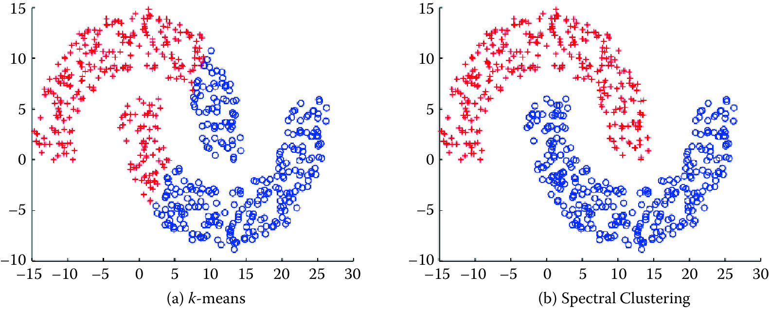
Figure 7.3: The same data set can produce drastically different clusters: (a) k-means; (b) spectral clustering
The algorithm works as follows:
Compute a similarity matrix from the data. This involves determining a pairwise distance function (using one of the distance functions we described earlier).
With this matrix, we can now perform graph partitioning, where connected graph components are interpreted as clusters. The graph must be partitioned such that edges connecting different clusters have low weights and edges within the same cluster have high values.
We can now partition these data represented by the similarity matrix in a variety of ways. One common way is to use the normalized cuts method. Another way is to compute a graph Laplacian from the similarity matrix.
Compute the eigenvectors and eigenvalues of the Laplacian.
The \(k\) eigenvectors are used as proxy data for the original data set, and they are fed into \(k\)-means clustering to produce cluster assignments for each original data point.
Spectral clustering is in general much better than \(k\)-means in clustering performance but much slower to run in practice. For large-scale problems, \(k\)-means is a preferred clustering algorithm to run because of efficiency and speed.
Principal components analysis
Principal components analysis is another unsupervised method used for finding patterns and structure in data. In contrast to clustering methods, the output is not a set of clusters but a set of principal components that are linear combinations of the original variables. PCA is typically used when you have a large number of variables and you want a reduced number that you can analyze. This approach is often called dimensionality reduction. It generates linearly uncorrelated dimensions that can be used to understand the underlying structure of the data. In mathematical terms, given a set of data on \(n\) dimensions, PCA aims to find a linear subspace of dimension \(d\) lower than \(n\) such that the data points lie mainly on this linear subspace.
PCA is related to several other methods you may already know about. Multidimensional scaling, factor analysis, and independent component analysis differ from PCA in the assumptions they make, but they are often used for similar purposes of dimensionality reduction and discovering the underlying structure in a data set.
Association rules
Association rules are a different type of analysis method and originate from the data mining and database community, primarily focused on finding frequent co-occurring associations among a collection of items. This method is sometimes referred to as “market basket analysis,” since that was the original application area of association rules. The goal is to find associations of items that occur together more often than you would randomly expect. The classic example (probably a myth) is “men who go to the store to buy diapers will also tend to buy beer at the same time.” This type of analysis would be performed by applying association rules to a set of supermarket purchase data. For social scientists, this method can be used on data that contains social services that individuals have received in the past to determine what types of services “co-occur” in people and proactively offer those services to people in need.
Association rules take the form \(X_1, X_2, X_3 \Rightarrow Y\) with support \(S\) and confidence \(C\), implying that when a transaction contains items \(\{X_1, X_2, X_3\}\) \(C\)% of the time, they also contain item \(Y\) and there are at least \(S\)% of transactions where the antecedent is true. This is useful in cases where we want to find patterns that are both frequent and statistically significant, by specifying thresholds for support \(S\) and confidence \(C\).
Support and confidence are useful metrics to generate rules but are often not enough. Another important metric used to generate rules (or reduce the number of spurious patterns generated) is lift. Lift is simply estimated by the ratio of the joint probability of two items, \(x\) and \(y\), to the product of their individual probabilities: \(P(x,y)/[P(x)P(y)]\). If the two items are statistically independent, then \(P(x,y)=P(x)P(y)\), corresponding to a lift of \(1\). Note that anti-correlation yields lift values less than 1, which is also an interesting pattern, corresponding to mutually exclusive items that rarely occur together.
Association rule algorithms work as follows: Given a set of transactions (rows) and items for that transaction:
Find all combinations of items in a set of transactions that occur with a specified minimum frequency. These combinations are called frequent itemsets.
Generate association rules that express co-occurrence of items within frequent itemsets.
For our purposes, association rule methods are an efficient way to take a basket of features (e.g., areas of publication of a researcher, different organizations an individual has worked at in their career, all the cities or neighborhoods someone may have lived in) and find co-occurrence patterns. This may sound trivial, but as data sets and number of features get larger, it becomes computationally expensive and association rule mining algorithms provide a fast and efficient way of doing it.
7.6.2 Supervised learning
We now turn to the problem of supervised learning, which typically involves methods for classification, prediction, and regression. We will mostly focus on classification methods in this chapter since many of the regression methods in machine learning are fairly similar to methods with which you are already familiar. Remember that classification means predicting a discrete (or categorical) variable. Most of the classification methods that we will cover can also be used for Regression (predicting continuous outcomes).
In general, supervised learning methods take as input pairs of data points \((X,Y)\) where \(X\) are the predictor variables (features) and \(Y\) is the target variable (label). The supervised learning method then uses these pairs as training data and learns a model \(F\), where \(F(X)\sim Y\). This model \(F\) is then used to predict \(Y\)s for new data points \(X\). As mentioned earlier, the goal is not to build a model that best fits known data but a model that is useful for future predictions and minimizes future generalization error. This is the key goal that differentiates many of the methods that you know from the methods that we will describe next. In order to minimize future error, we want to build models that are not just overfitting on past data.
Another goal, often prioritized in the social sciences, that machine learning methods do not optimize for is getting a structural form of the model. Machine learning models for classification can take different structural forms (ranging from linear models, to sets of rules, to more complex non-linear forms), and it may not always be possible to write them down in a compact form as an equation. This does not, however, make them incomprehensible or uninterpretable. Another focus of machine learning models for supervised learning is prediction, and not necessarily causal inference57. Some of these models can be used to help with causal inference, but they are typically optimized for prediction tasks. We believe that there are many social science and policy problems where better prediction methods can be extremely beneficial (Kleinberg et al. 2015).
In this chapter, we mostly deal with binary classification problems: that is, problems in which the data points are to be classified into one of two categories. Several of the methods that we will cover can also be used for multiclass classification (classifying a data point into one of \(n\) categories) or for multi-label classification (classifying a data point into \(m\) of \(n\) categories where \(m\ge1\)). There are also approaches to take multiclass problems and turn them into a set of binary problems that we will mention briefly in the next section.
Before we describe supervised learning methods, we want to recap a few principles as well as terms that we have used and will be using in the rest of the chapter.
Training a model
Once we have finished data exploration, filled in missing values, created predictor variables (features), and decided what our target variable (label) is, we now have pairs of \(X,Y\) to start training (or building) the model.
Using the model to score new data
We are building this model so we can predict \(Y\) for a new set of \(X\)s—using the model means, getting new data, generating the same features to get the vector \(X\), and then applying the model to produce \(Y\).
One common technique for supervised learning is logistic regression, a method you will already be familiar with. We will give an overview of some of the other methods used in machine learning. It is important to remember that as you use increasingly powerful classification methods, you need more data to train the models.
\(k\)-nearest neighbor
The method \(k\)-nearest neighbor (\(k\)-NN) is one of the simpler classification methods in machine learning. It belongs to a family of models sometimes known as memory-based models or instance-based models. An example is classified by finding its \(k\) nearest neighbors and taking majority vote (or some other aggregation function). We need two key things: a value for \(k\) and a distance metric with which to find the \(k\) nearest neighbors. Typically, different values of \(k\) are used to empirically find the best one. Small values of \(k\) lead to predictions having high variance but can capture the local structure of the data. Larger values of \(k\) build more global models that are lower in variance but may not capture local structure in the data as well.
Figure 7.4 provides an example for \(k = 1, 3, 5\) nearest neighbors. The number of neighbors (\(k\)) is a parameter, and the prediction depends heavily on how it is determined. In this example, point B is classified differently if \(k = 3\).
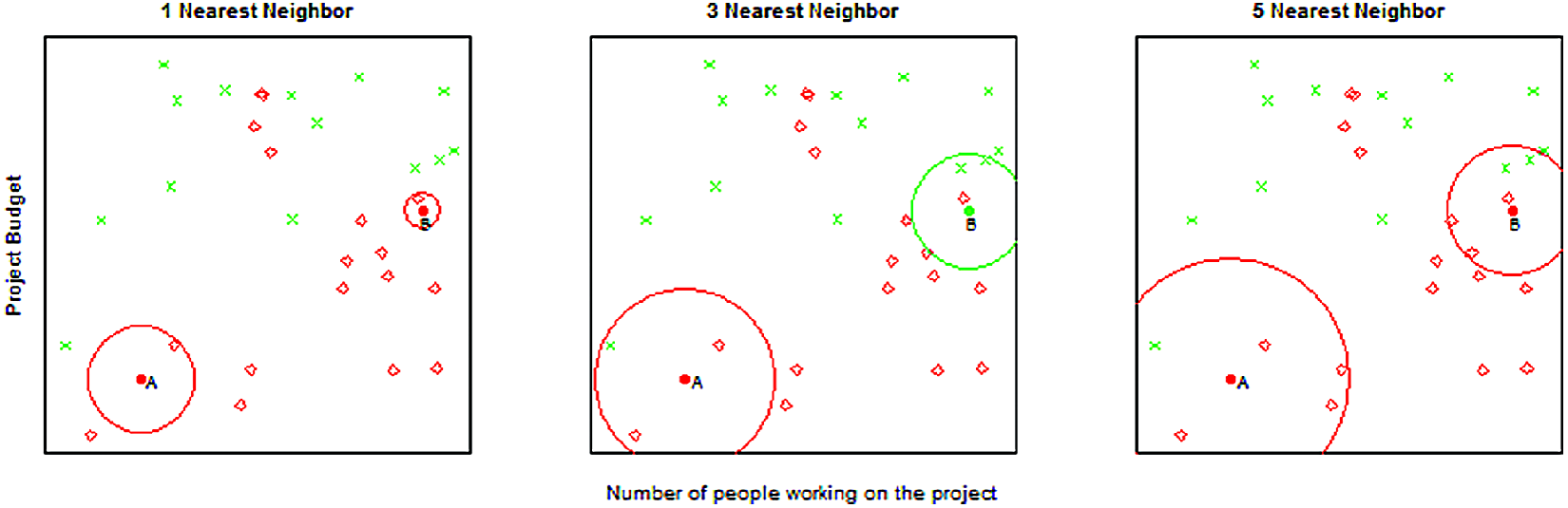
Figure 7.4: Example of \(k\)-nearest neighbor with \(k = 1, 3, 5\) neighbors. We want to predict the points A and B. The 1-nearest neighbor for both points is red (“Patent not granted”), the 3-nearest neighbor predicts point A (B) to be red (green) with probability 2/3, and the 5-nearest neighbor predicts again both points to be red with probabilities 4/5 and 3/5, respectively.
Training for \(k\)-NN just means storing the data, making this method useful in applications where data are coming in extremely quickly and a model needs to be updated frequently. All the work, however, gets pushed to scoring time, since all the distance calculations happen when a new data point needs to be classified. There are several optimized methods designed to make \(k\)-NN more efficient that are worth looking into if that is a situation that is applicable to your problem.
In addition to selecting \(k\) and an appropriate distance metric, we also have to be careful about the scaling of the features. When distances between two data points are large for one feature and small for a different feature, the method will rely almost exclusively on the first feature to find the closest points. The smaller distances on the second feature are nearly irrelevant to calculate the overall distance. A similar problem occurs when continuous and categorical predictors are used together. To resolve the scaling issues, various options for rescaling exist. For example, a common approach is to center all features at mean \(0\) and scale them to variance \(1\).
There are several variations of \(k\)-NN. One of these is weighted nearest neighbors, where different features are weighted differently or different examples are weighted based on the distance from the example being classified. The method \(k\)-NN also has issues when the data are sparse and has high dimensionality, which means that every point is far away from virtually every other point, and hence pairwise distances tend to be uninformative. This can also happen when a lot of features are irrelevant and drown out the relevant features’ signal in the distance calculations.
Notice that the nearest-neighbor method can easily be applied to regression problems with a real-valued target variable. In fact, the method is completely oblivious to the type of target variable and can potentially be used to predict text documents, images, and videos, based on the aggregation function after the nearest neighbors are found.
Support vector machines
Support vector machines are one of the most popular and best-performing classification methods in machine learning today. The mathematics behind SVMs has a lot of prerequisites that are beyond the scope of this book, but we will give you an intuition of how SVMs work, what they are good for, and how to use them.
We are all familiar with linear models (e.g., logistic regression) that separate two classes by fitting a line in two dimensions (or a hyperplane in higher dimensions) in the middle (see Figure 7.5). An important decision that linear models have to make is which linear separator we should prefer when there are several we can build.
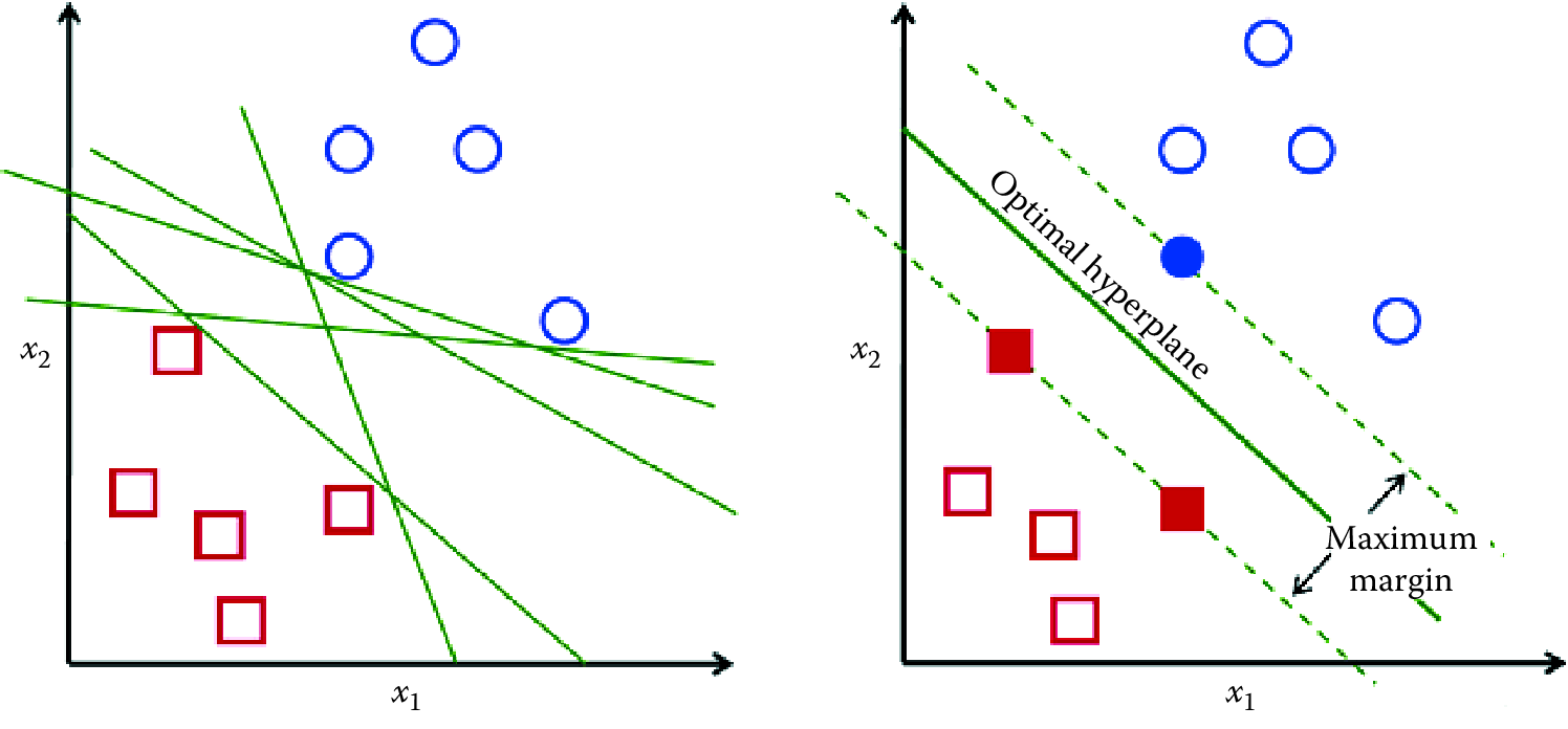
Figure 7.5: Support vector machines
You can see in Figure 7.5 that multiple lines offer a solution to the problem. Is any of them better than the others? We can intuitively define a criterion to estimate the worth of the lines: A line is bad if it passes too close to the points because it will be noise sensitive and it will not generalize correctly. Therefore, our goal should be to find the line passing as far as possible from all points.
The SVM algorithm is based on finding the hyperplane that maximizes the margin of the training data. The training examples that are closest to the hyperplane are called support vectors since they are supporting the margin (as the margin is only a function of the support vectors).
An important concept to learn when working with SVMs is kernels. SVMs are a specific instance of a class of methods called kernel methods. So far, we have only talked about SVMs as linear models. Linear works well in high-dimensional data but sometimes you need nonlinear models, often in cases of low-dimensional data or in image or video data. Unfortunately, traditional ways of generating nonlinear models get computationally expensive since you have to explicitly generate all the features such as squares, cubes, and all the interactions. Kernels are a way to keep the efficiency of the linear machinery but still build models that can capture nonlinearity in the data without creating all the nonlinear features.
You can essentially think of kernels as similarity functions and use them to create a linear separation of the data by (implicitly) mapping the data to a higher-dimensional space. Essentially, we take an \(n\)-dimensional input vector \(X\), map it into a high-dimensional (infinite-dimensional) feature space, and construct an optimal separating hyperplane in this space. We refer you to relevant papers for more detail on SVMs and nonlinear kernels (Shawe-Taylor and Cristianini 2004; Scholkopf and Smola 2001). SVMs are also related to logistic regression, but use a different loss/penalty function (Hastie, Tibshirani, and Friedman 2001).
When using SVMs, there are several parameters you have to optimize, ranging from the regularization parameter \(C\), which determines the tradeoff between minimizing the training error and minimizing model complexity, to more kernel-specific parameters. It is often a good idea to do a grid search to find the optimal parameters. Another tip when using SVMs is to normalize the features; one common approach to doing that is to normalize each data point to be a vector of unit length.
Linear SVMs are effective in high-dimensional spaces, especially when the space is sparse such as text classification where the number of data points (perhaps tens of thousands) is often much less than the number of features (a hundred thousand to a million or more). SVMs are also fairly robust when the number of irrelevant features is large (unlike the \(k\)-NN approaches that we mentioned earlier) as well as when the class distribution is skewed, that is, when the class of interest is significantly less than 50% of the data.
One disadvantage of SVMs is that they do not directly provide probability estimates. They assign a score based on the distance from the margin. The farther a point is from the margin, the higher the magnitude of the score. This score is good for ranking examples, but getting accurate probability estimates takes more work and requires more labeled data to be used to perform probability calibrations.
In addition to classification, there are also variations of SVMs that can be used for regression (Smola and Schölkopf 2004) and ranking (Chapelle and Keerthi 2010).
Decision trees
Decision trees are yet another set of methods that are helpful for prediction. Typical decision trees learn a set of rules from training data represented as a tree. An exemplary decision tree is shown in Figure 7.6. Each level of a tree splits the tree to create a branch using a feature and a value (or range of values). In the example tree, the first split is made on the feature number of visits in the past year and the value \(4\). The second level of the tree now has two splits: one using average length of visit with value \(2\) days and the other using the value \(10\) days.
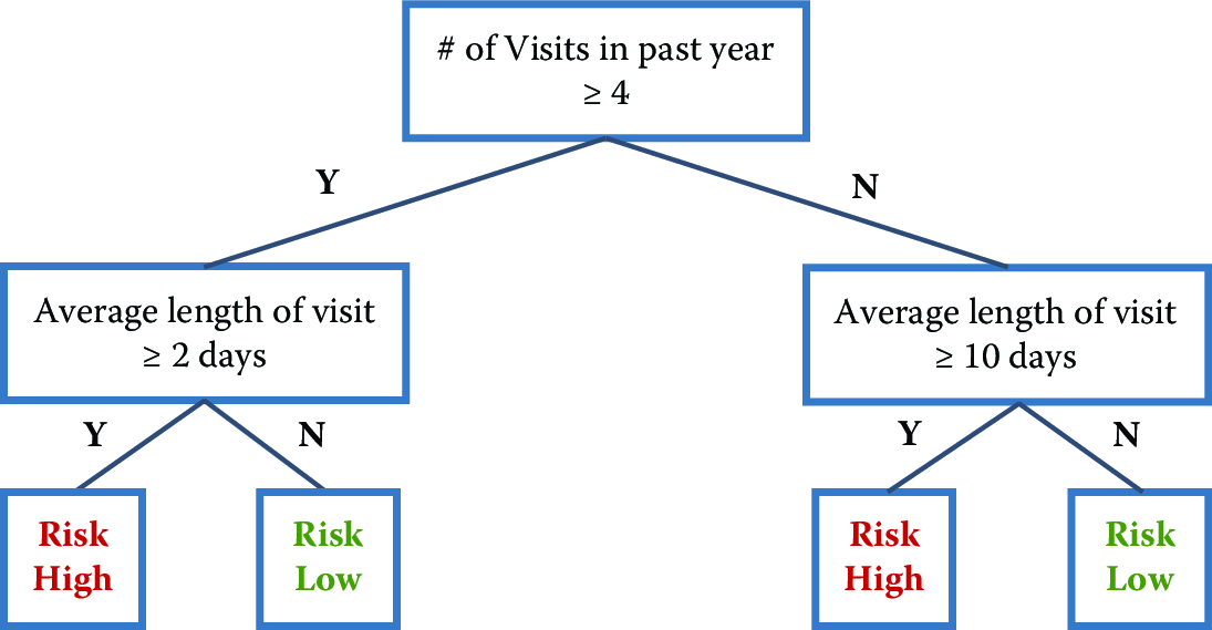
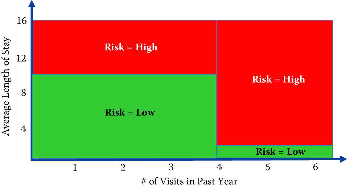
Figure 7.6: An exemplary decision tree. The top figure is the standard representation for trees. The bottom figure offers an alternative view of the same tree. The feature space is partitioned into numerous rectangles, which is another way to view a tree, representing its nonlinear character more explicitly
Various algorithms exist to build decision trees. C4.5, CHAID, and CART (Classification and Regression Trees) are the most popular. Each needs to determine the next best feature to split on. The goal is to find feature splits that can best reduce class impurity in the data, that is, a split that will ideally put all (or as many as possible) positive class examples on one side and all (or as many as possible) negative examples on the other side. One common measure of impurity that comes from information theory is entropy, and it is calculated as \[H(X) = -\sum_x p(x) \log p(x).\]
Entropy is maximum (1) when both classes have equal numbers of examples in a node. It is minimum (0) when all examples are from the same class. At each node in the tree, we can evaluate all the possible features and select the one that most reduces the entropy given the tree so far. This expected change in entropy is known as information gain and is one of the most common criteria used to create decision trees. Other measures that are used instead of information gain are Gini and chi-squared.
If we keep constructing the tree in this manner, selecting the next best feature to split on, the tree ends up fairly deep and tends to overfit the data. To prevent overfitting, we can either have a stopping criterion or prune the tree after it is fully grown. Common stopping criteria include minimum number of data points to have before doing another feature split, maximum depth, and maximum purity. Typical pruning approaches use holdout data (or cross-validation, which will be discussed later in this chapter) to cut off parts of the tree.
Once the tree is built, a new data point is classified by running it through the tree and, once it reaches a terminal node, using some aggregation function to give a prediction (classification or regression). Typical approaches include performing maximum likelihood (if the leaf node contains 10 examples, 8 positive and 2 negative, any data point that gets into that node will get an 80% probability of being positive). Trees used for regression often build the tree as described above but then fit a linear regression model at each leaf node.
Decision trees have several advantages. The interpretation of a tree is straightforward as long as the tree is not too large. Trees can be turned into a set of rules that experts in a particular domain can possibly dig deeper into, validate, and modify. Trees also do not require too much feature engineering. There is no need to create interaction terms since trees can implicitly do that by splitting on two features, one after another.
Unfortunately, along with these benefits come a set of disadvantages. Decision trees, in general, do not perform well, compared to SVMs, random forests, or logistic regression. They are also unstable: small changes in data can result in very different trees. The lack of stability comes from the fact that small changes in the training data may lead to different splitting points. As a consequence, the whole tree may take a different structure. The suboptimal predictive performance can be seen from the fact that trees partition the predictor space into a few rectangular regions, each one predicting only a single value (see the bottom part of Figure 7.6.
Ensemble methods
Combinations of models are generally known as model ensembles. They are among the most powerful techniques in machine learning, often outperforming other methods, although at the cost of increased algorithmic and model complexity.
The intuition behind building ensembles of models is to build several models, each somewhat different. This diversity can come from various sources such as: training models on subsets of the data; training models on subsets of the features; or a combination of these two.
Ensemble methods in machine learning have two things in common. First, they construct multiple, diverse predictive models from adapted versions of the training data (most often reweighted or resampled). Second, they combine the predictions of these models in some way, often by simple averaging or voting (possibly weighted).
Bagging
Bagging stands for “bootstrap aggregation”58: we first create bootstrap samples from the original data and then aggregate the predictions using models trained on each bootstrap sample. Given a data set of size \(N\), the method works as follows:
Create \(k\) bootstrap samples (with replacement), each of size \(N\), resulting in \(k\) data sets. Only about 63% of the original training examples will be represented in any given bootstrapped set.
Train a model on each of the \(k\) data sets, resulting in \(k\) models.
For a new data point \(X\), predict the output using each of the \(k\) models.
Aggregate the \(k\) predictions (typically using average or voting) to get the prediction for \(X\).
A nice feature of this method is that any underlying model can be used, but decision trees are often the most commonly used base model. One reason for this is that decision trees are typically high variance and unstable, that is, they can change drastically given small changes in data, and bagging is effective at reducing the variance of the overall model. Another advantage of bagging is that each model can be trained in parallel, making it efficient to scale to large data sets.
Boosting
Boosting is another popular ensemble technique, and it often results in improving the base classifier being used. In fact, if your only goal is improving accuracy, you will most likely find that boosting will achieve that. The basic idea is to keep training classifiers iteratively, each iteration focusing on examples that the previous one got wrong. At the end, you have a set of classifiers, each trained on smaller and smaller subsets of the training data. Given a new data point, all the classifiers predict the target, and a weighted average of those predictions is used to get the final prediction, where the weight is proportional to the accuracy of each classifier. The algorithm works as follows:
Assign equal weights to every example.
For each iteration:
Train classifier on the weighted examples.
Predict on the training data.
Calculate error of the classifier on the training data.
Calculate the new weighting on the examples based on the errors of the classifier.
Reweight examples.
Generate a weighted classifier based on the accuracy of each classifier.
One constraint on the classifier used within boosting is that it should be able to handle weighted examples (either directly or by replicating the examples that need to be overweighted). The most common classifiers used in boosting are decision stumps (single-level decision trees), but deeper trees can also work well.
Boosting is a common way to boost the performance of a classification method but comes with additional complexity, both in the training time and in interpreting the predictions. A disadvantage of boosting is that it is difficult to parallelize since the next iteration of boosting relies on the results of the previous iteration.
A nice property of boosting is its ability to identify outliers: examples that are either mislabeled in the training data, or are inherently ambiguous and hard to categorize. Because boosting focuses its weight on the examples that are more difficult to classify, the examples with the highest weight often turn out to be outliers. On the other hand, if the number of outliers is large (lots of noise in the data), these examples can hurt the performance of boosting by focusing too much on them.
Random forests
Given a data set of size \(N\) and containing \(M\) features, the random forest training algorithm works as follows:
Create \(n\) bootstrap samples from the original data of size \(N\). Remember, this is similar to the first step in bagging. Increasing \(n\) will lead to similar or better results, but also requires more computational resources. Typically \(n\) ranges from 100 to a few thousand but is best determined empirically.
For each bootstrap sample, train a decision tree using \(m\) features (where \(m\) is typically much smaller than \(M\)) at each node of the tree. The \(m\) features are selected uniformly at random from the \(M\) features in the data set, and the decision tree will select the best split among the \(m\) features. The value of \(m\) is held constant during the forest growing.
A new test example/data point is classified by all the trees, and the final classification is done by majority vote (or another appropriate aggregation method).
Random forests often achieve remarkable results while being simple to use. They can be easily parallelized, making them efficient to run on large data sets, and can handle a large number of features, even with a lot of missing values. Random forests can get complex, with hundreds or thousands of trees that are fairly deep, so it is difficult to interpret the learned model. At the same time, they provide a nice way to estimate feature importance, giving a sense of what features were important in building the classifier.
Another nice aspect of random forests is the ability to compute a proximity matrix that gives the similarity between every pair of data points. This is calculated by computing the number of times two examples land in the same terminal node. The more that happens, the closer the two examples are. We can use this proximity matrix for clustering, locating outliers, or explaining the predictions for a specific example.
Stacking
Stacking is a technique that deals with the task of learning a meta-level classifier to combine the predictions of multiple base-level classifiers. This meta-algorithm is trained to combine the model predictions to form a final set of predictions. This can be used for both regression and classification. The algorithm works as follows:
Split the data set into \(n\) equal-sized sets: \(set_1, set_2,\ldots,set_n\).
Train base models on all possible combinations of \(n-1\) sets and, for each model, use it to predict on \(set_i\) what was left out of the training set. This would give us a set of predictions on every data point in the original data set.
Now train a second-stage stacker model on the predicted classes or the predicted probability distribution over the classes from the first-stage (base) model(s).
By using the first-stage predictions as features, a stacker model gets more information on the problem space than if it were trained in isolation. The technique is similar to cross-validation, an evaluation methodology that we will cover later in this chapter.
Neural networks and deep learning
Neural networks are a set of multi-layer classifiers where the outputs of one layer feed into the inputs of the next layer. The layers between the input and output layers are called hidden layers, and the more hidden layers a neural network has, the more complex functions it can learn. Neural networks were popular in the 1980s and early 1990s, but then fell out of fashion because they were slow and expensive to train, even with only one or two hidden layers. Since 2006, a set of techniques has been developed that enable learning in deeper neural networks. These techniques, with access to massive computational resources and large amounts of data, have enabled much deeper (and larger) networks to be Trained and it turns out that these perform far better on many problems than shallow neural networks (with just a single hidden layer). The reason for the better performance is the ability of deep nets to build up a complex hierarchy of concepts, learning multiple levels of representation and abstraction that help to make sense of data such as images, sound, and text.
There are a few different types of neural networks that are popular today:
Convolutional Neural Networks (CNNs): These are often used in detecting objects in images and in doing image search, but their applicability goes beyond just image analysis and they can be used to find patterns in other types of data as well. CNNs treat input data (such as images) in a spatial manner (in two or three dimensions for example), and are able to capture spatial dependencies in the data.
Recurrent Neural Networks (RNNs): are suitable for modeling sequential data that has temporal dependencies. They are trained to generate the next steps in a sequence, such as the next letters in a word, or the next words in a sentence, voice recording, or video. They are typically used in translation, speech generation, and time series prediction tasks. A popular variation of RNNs is LSTM (Long Short Term Memory) that are used because of their ability and effectiveness in modeling long-range dependencies.
Generative Adversarial Network (GANs): have been shown to be quite adept at generating new, realistic images based on other training images. GANs train two models in parallel. One network (called generator) is trained to generate data (based on historical examples of previously occurring data such as images or text or video). The other network (discriminator) tries to classify these generated images as real or synthetic. During training a GAN, the goal is to generate data that is realistic enough that the discriminator network is fooled to the point that it cannot distinguish the difference between the real and the synthetic input data.
Goodfellow et al. (2016) provide a (mathematical) introduction to deep learning.
Currently, deep neural networks are popular for a certain class of problems and a lot of research is being done on them. It is, however, important to keep in mind that they may often require a lot more data than are available in many problems. In many problems, such as natural language processing, image, and video analysis, there are techniques to start from a pre-trained neural network model, that reduces the need for additional training data. Training deep neural networks also requires a lot of computational power, but that is less likely to be an issue for most people today with increased access to computing resources. Typical cases where deep learning has been shown to be effective involve lots of images, video, and text data. We are in the early stages of development of this class of methods, and although there seems to be a lot of potential, we need a much better understanding of why they are effective and the problems for which they are well suited.
7.6.3 Binary vs Multiclass classification problems
In the discussion above, we framed classification problems as binary classification problems with a 0 or 1 output. There are many problems where we have multiple classes, such as classifying companies into their industry codes or predicting whether a student will drop out, transfer, or graduate. Several solutions have been designed to deal with the multiclass classification problem:
Direct multiclass: Use methods that can directly perform multiclass classification. Examples of such methods are \(K\)-nearest neighbor, decision trees, and random forests. There are extensions of support vector machines that exist for multiclass classification as well (Crammer and Singer 2002), but they can often be slow to train.
Convert to one versus all (OVA): This is a common approach to solve multiclass classification problems using binary classifiers. Any problem with \(n\) classes can be turned into \(n\) binary classification problems, where each classifier is trained to distinguish between one versus all the other classes. A new example can be classified by combining the predictions from all the \(n\) classifiers and selecting the class with the highest score. This is a simple and efficient approach, and one that is commonly used, but it suffers from each classification problem possibly having an imbalanced class distribution (due to the negative class being a collection of multiple classes). Another limitation of this approach is that it requires the scores of each classifier to be calibrated so that they are comparable across all of them.
Convert to pairwise: In this approach, we can create binary classifiers to distinguish between each pair of classes, resulting in \(\binom{n}{2}\) binary classifiers. This results in a large number of classifiers, but each classifier usually has a balanced classification problem. A new example is classified by taking the predictions of all the binary classifiers and using majority voting.
7.6.4 Skewed or imbalanced classification problems
A lot of problems you will deal with will not have uniform (balanced) distributions for both classes. This is often the case with problems in fraud detection, network security, and medical diagnosis where the class of interest is not very common. The same is true in many social science and public policy problems around behavior prediction, such as predicting which students will not graduate on time, which children may be at risk of getting lead poisoning, or which homes are likely to be abandoned in a given city. You will notice that applying standard machine learning methods may result in all the predictions being for the most frequent category in such situations, making it problematic to detect the infrequent classes. There has been a lot of work in machine learning research on dealing with such problems (Chawla 2005; Kuhn and Johnson 2013) that we will not cover in detail here. Common approaches to deal with class imbalance include oversampling from the minority class and undersampling from the majority class. It is important to keep in mind that the sampling approaches do not need to result in a \(1:1\) ratio. Many supervised learning methods described in this chapter (such as Random Forests and SVMs) can work well even with a \(10:1\) imbalance. Also, it is critical to make sure that you only resample the training set; keep the distribution of the test set the same as that of the original data since you will not know the class labels of new data in practice and will not be able to resample.
7.6.5 Model interpretability
As social scientists (or good machine learning practitioners), we do not only care about building machine learning models but also want to understand what the models “learned”, and how to use them to make inferences and decisions. Understanding, or interpreting machine learning models is a key requirement for most social science and policy problems. There are various reasons for this including:
- Providing information that can help in debugging and improving models
- Increasing trust in the models and hence increasing their adoption by decisionmakers
- Improving the decisions being made using the models by reinforcing the correct predictions and helping the decision-maker override the wrong predictions.
- Helping select appropriate interventions based on the explanations
- Providing legal recourse to people being affected by the decisions made using the models
Global versus Individual-Level Explanations
When thinking about model interpretability, there are two types of interpretability:
- Global: At the overall model level
- Individual: Explaining an individual classification/prediction that is made by a model.
Both of these are important for different reasons. We need global interpretability to help understand the overall model but we also need explanations for individual classifications when these models are helping a person make decisions about individual cases. A social worker identifying the risk of a client going back to the homeless shelter and determining appropriate interventions to reduce that risk, or a counselor in an employment agency determining how likely an individual is to be long-term unemployed and connecting them with appropriate training programs or job opportunities need individual-level explanations of predictions/recommendations that the machine learning model is generating.
Global Interpretability
Each method results in a model that needs to be interpreted in a way that is appropriate for that method. For example, for a decision tree, we may want to view the tree to understand what types of classifications are being made. This can of course get cumbersome and difficult if the tree is extremely large. For logistic regression models, we can look at the coefficients and odds-ratios, but it is often difficult to mentally account for different variables controlling for each other. In general, the models discussed above have different ways of exposing their “feature importances”^[Some measure of how useful that feature was for the given model.] and we often use that as a proxy for global model interpretability.
Another way of interpreting a model is to understand how the model scores individual data points. We can take the set of entities that are scored by the model, and generate cross-tabs that highlight how the top x% of the scored/predicted entities are different from the rest of the entities. This approach allows us to get an idea of what the model is doing, not in general, but on the entities of interest to us and makes interpretability a little more intuitive and generalizable across different model types.
A different approach that some have taken in this area has been to sparse^[Using a small number of features/predictors.] models, making them easier to interpret. The motivation behind these simple, sparse models is that they are inherently interpretable and do not require the use of additional analysis for humans to understand them. Examples of such work include Ustun and Rudin (2019), Ustun and Rudin (2016), and Caruana et al. (2015). These models may not perform well in every task so it’s important for us to explore the range of models in terms of performance and complexity, and decide what level and type of interpretability we need and how to balance that with the accuracy59 of those models.
Individual-Level Explanations
While it’s important to understand the models we are building at a global level, in many social science applications, we want to get an explanation for why a data point was classified/predicted a certain way by the model. There has been a lot of recent work on methods for generating individual-level explanations for predictions made by machine learning models. These fall into two areas: 1. Model specific methods: These are used to generate explanations for predictions made by a specific class of methods, such as neural networks or random forests. 2. Model agnostic methods: These can be used to generate explanations for individual predictions made by any type of model. Examples of this include LIME (Ribeiro, Singh, and Guestrin 2016), MAPLE (Plumb, Molitor, and Talwalkar 2018), and SHAP values (Lundberg and Lee 2017).
It’s important to keep in mind though that these “explanations” are typically not causal, and are often restricted to be a ranked list of “features”. One way to think about them is that these features were most important in assigning this data point the score it was given by a particular model. This is currently an active area of machine learning research and will hopefully mature into a set of methods and tools useful for social scientists using machine learning to solve problems that require a better and deeper understanding of their predictions.
7.7 Evaluation
The previous section introduced us to a variety of methods, all with certain pros and cons, and no single method guaranteed to outperform others for a given problem. This section focuses on evaluation methods, with three primary goals:
Model selection: How do we select a method to use in the future? What parameters should we select for that method?
Performance estimation: How do we estimate how well our model will perform once it is deployed and applied to new data?
A deeper understanding of the types of models that work well and those that don’t can point to the effectiveness and applicability of existing methods and provide a better understanding of the structure of the data and the problem we are tackling.
This section will cover evaluation methodologies as well as metrics that are commonly used.
7.7.1 Methodology
In-sample evaluation
As social scientists, you already evaluate methods on how well they perform in-sample (on the set that the model was trained on). As we mentioned earlier in the chapter, the goal of machine learning methods is to generalize to new data, and validating models in-sample does not allow us to do that. We focus here on evaluation methodologies that allow us to optimize (as best as we can) for generalization performance. The methods are illustrated in Figure 7.7.
Out-of-sample and holdout set
The simplest way to focus on generalization is to pretend to generalize to new (unseen) data. One way to do that is to take the original data and randomly split them into two sets: a training set and a test set (sometimes also called the holdout or validation set). We can decide how much to keep in each set (typically the splits range from 50–50 to 80–20, depending on the size of the data set). We then train our models on the training set and classify the data in the test set, allowing us to get an estimate of the relative performance of the methods.
One drawback of this approach is that we may be extremely lucky or unlucky with our random split. One way to get around the problem that is to repeatedly create multiple training and test sets. We can then train on \(TR_1\) and test on \(TE_1\), train on \(TR_2\) and test on \(TE_2\), and so on. The performance measures on each test set can then give us an estimate of the performance of different methods and how much they vary across different random sets.
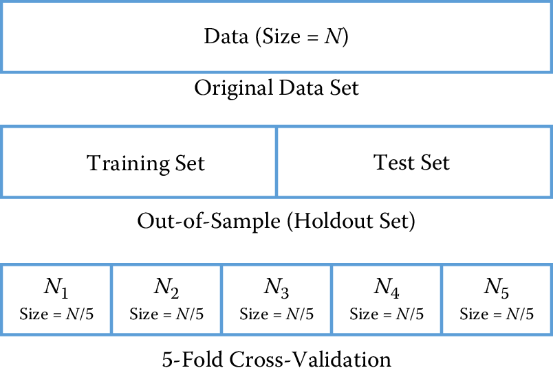
Figure 7.7: Validation methodologies: holdout set and cross-validation
Cross-validation
Cross-validation is a more sophisticated holdout training and testing procedure that takes away some of the shortcomings of the holdout set approach. Cross-validation begins by splitting a labeled data set into \(k\) partitions (called folds). Typically, \(k\) is set to \(5\) or \(10\). Cross-validation then proceeds by iterating \(k\) times. In each iteration, one of the \(k\) folds is held out as the test set, while the other \(k-1\) folds are combined and used to train the model. A nice property of cross-validation is that every example is used in one test set for testing the model. Each iteration of cross-validation gives us a performance estimate that can then be aggregated (typically averaged) to generate the overall estimate.
An extreme case of cross-validation is called leave-one-out cross-validation, where given a data set of size \(N\), we create \(N\) folds. That means iterating over each data point, holding it out as the test set, and training on the rest of the \(N-1\) examples. This illustrates the benefit of cross-validation by giving us good generalization estimates (by training on as much of the data set as possible) and making sure the model is tested on each data point.
Temporal validation
The cross-validation and holdout set approaches described above assume that the data have no time dependencies and that the distribution is stationary over time. This assumption is almost always violated in practice and affects performance estimates for a model.
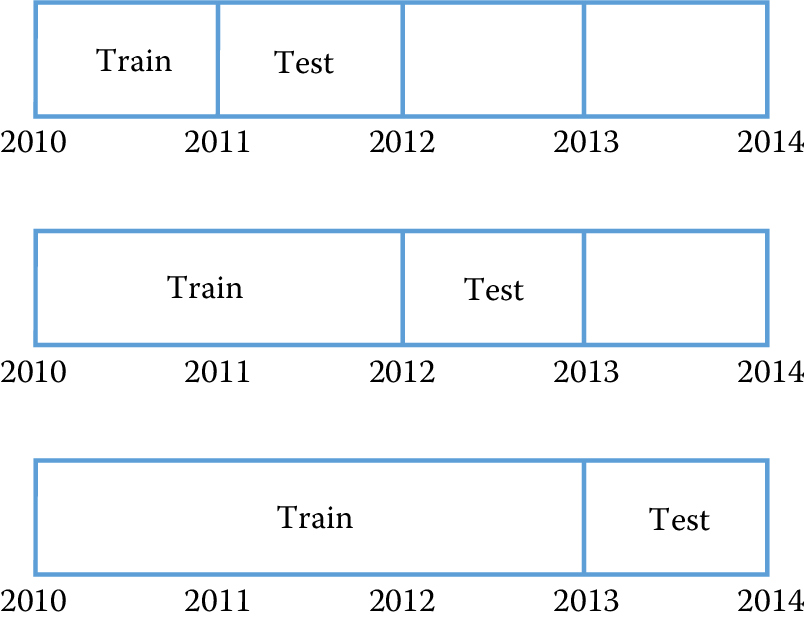
Figure 7.8: Temporal validation
In most practical problems, we want to use a validation strategy that emulates the way in which our models will be used and provides an accurate performance estimate. We will call this temporal validation. For a given point in time \(t_i\), we train our models only on information available to us before \(t_i\) to avoid training on data from the “future.” We then predict and evaluate on data from \(t_i\) to \(t_i\) + \(d\) and iterate, expanding the training window while keeping the test window size constant at \(d\). Figure 7.8 shows this validation process with \(t_i=2010\) and \(d=1\) year. The test set window \(d\) depends on a few factors related to how the model will be deployed to best emulate reality:
How far out in the future do predictions need to be made? For example, if the set of students who need to be targeted for interventions has to be finalized at the beginning of the school year for the entire year, then \(d = 1\) year.
How often will the model be updated? If the model is being updated daily, then we can move the window by a day at a time to reflect the deployment scenario.
How often will the system get new data? If we are getting new data frequently, we can make predictions more frequently.
Temporal validation is similar to how time series models are evaluated (also known as backtesting) and should be the validation approach used for most practical problems.
7.7.2 Metrics
The previous subsection focused on validation methodologies assuming we have an evaluation metric in mind. This section will go over commonly used evaluation metrics. You are probably familiar with using \(R^2\), analysis of the residuals, and mean squared error (MSE) to evaluate the quality of regression models. For regression problems, the MSE calculates the average squared differences between predictions \(\hat{y}_i\) and true values \(y_i\). When prediction models have smaller MSE, they are better. However, the MSE itself is hard to interpret because it measures quadratic differences. Instead, the root mean squared error (RMSE) is more intuitive as it as measure of mean differences on the original scale of the response variable. Yet another alternative is the mean absolute error (MAE), which measures average absolute distances between predictions and true values.
We will now describe some additional evaluation metrics commonly used in machine learning for classification. Before we dive into metrics, it is important to highlight that machine learning models for classification typically do not predict 0/1 values directly. SVMs, random forests, and logistic regression all produce a score (which is sometimes a probability) that is then turned into 0 or 1 based on a user-specific threshold. You might find that certain tools (such as scikit-learn60) use a default value for that threshold (often 0.5), but it is important to know that it is an arbitrary threshold and you should select the threshold based on the data, the model, and the problem you are solving. We will cover that a little later in this section.
Once we have turned the real-valued predictions into 0/1 classification, we can now create a confusion matrix from these predictions, shown in Figure 7.9. Each data point belongs to either the positive class or the negative class, and for each data point the prediction of the classifier is either correct or incorrect. This is what the four cells of the confusion matrix represent. We can use the confusion matrix to describe several commonly used evaluation metrics.
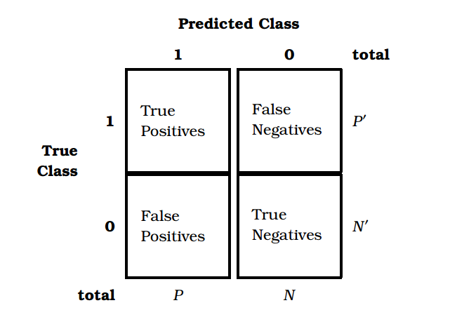
Figure 7.9: A confusion matrix created from real-valued predictions
Accuracy is the ratio of correct predictions (both positive and negative) to all predictions: \[\textrm{Accuracy}=\frac{TP + TN}{TP + TN + FP + FN}=\frac{TP + TN}{P+N}=\frac{TP + TN}{P'+N'},\] where \(TP\) denotes true positives, \(TN\) true negatives, \(FP\) false positives, \(FN\) false negatives, and other symbols denote row or column totals. Accuracy is the most commonly described evaluation metric for classification but is surprisingly the least useful in practical situations (at least by itself). One problem with accuracy is that it does not give us an idea of lift compared to baseline. For example, if we have a classification problem with 95% of the data as positive and 5% as negative, a classifier with 85% is performing worse than a dumb classifier that predicts positive all the time (and will have 95% accuracy).
Two additional metrics that are often used are precision and recall, which are defined as follows: \[\begin{aligned} {\rm Precision} &= \frac{TP}{TP + FP}=\frac{TP}{P}, \\ {\rm Recall} &= \frac{TP}{TP + FN}=\frac{TP}{P'} \end{aligned}\] (see also Box Vocabulary). Precision measures the accuracy of the classifier when it predicts an example to be positive. It is the ratio of correctly predicted positive examples (\(TP\)) to all examples predicted as positive (\(TP + FP\)). This measure is also called positive predictive value in other fields. Recall measures the ability of the classifier to find positive examples. It is the ratio of all the correctly predicted positive examples (\(TP\)) to all the positive examples in the data (\(TP + FN\)). This is also called sensitivity in other fields.
You might have encountered another metric called specificity in other fields. This measure is the true negative rate: the proportion of negatives that are correctly identified.
Another metric that is used is the \(F_1\) score, which is the harmonic mean of precision and recall: \[F_1 = \frac{2* {\rm Precision} * {\rm Recall}}{{\rm Precision} + {\rm Recall}}\]
This is often used when you want to balance both precision and recall.
There is often a tradeoff between precision and recall. By selecting different classification thresholds, we can vary and tune the precision and recall of a given classifier. A highly conservative classifier that only predicts a 1 when it is absolutely sure (say, a threshold of 0.9999) will most often be correct when it predicts a 1 (high precision) but will miss most 1s (low recall). At the other extreme, a classifier that says 1 to every data point (a threshold of 0.0001) will have perfect recall but low precision. Figure 7.10 show a precision–recall curve that is often used to represent the performance of a given classifier.
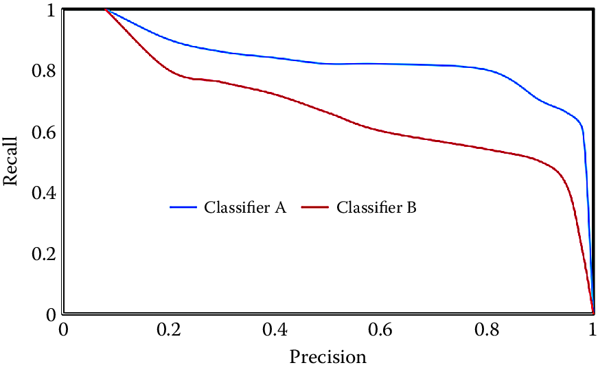
Figure 7.10: Precision–recall curve
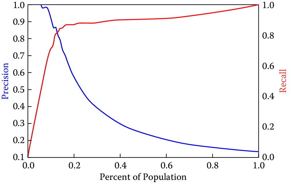
Figure 7.11: Precision or recall at different thresholds
If we care about optimizing for the entire precision recall space, a useful metric is the area under the curve (AUC-PR), which is the area under the precision–recall curve. AUC-PR must not be confused with AUC-ROC, which is the area under the related receiver operating characteristic (ROC) curve. The ROC curve is created by plotting recall versus (1 – specificity). Both AUCs can be helpful metrics to compare the performance of different methods and the maximum value the AUC can take is 1. If, however, we care about a specific part on the precision–recall curve, we have to look at finer-grained metrics.
Let us consider an example from public health. Most public health agencies conduct inspections of various sorts to detect health hazard violations (lead hazards, for example). The number of possible places (homes or businesses) to inspect far exceeds the inspection resources typically available. Let us assume further that they can only inspect 5% of all possible places; they would clearly want to prioritize the inspection of places that are most likely to contain the hazard. In this case, the model will score and rank all the possible inspection places in order of hazard risk. We would then want to know what percentage of the top 5% (the ones that will get inspected) are likely to be hazards, which translates to the precision in the top 5% of the most confidence predictions—precision at 5%, as it is commonly called (see Figure 7.11). Precision at top k percent is a common class of metrics widely used in information retrieval and search engine literature, where you want to make sure that the results retrieved at the top of the search results are accurate. More generally, this metric is often used in problems in which the class distribution is skewed and only a small percentage of the examples will be examined manually (inspections, investigations for fraud, etc.). The literature provides many case studies of such applications (Kumar, Ghani, and Mei 2010; Lakkaraju et al. 2015; Potash et al. 2015).
One last metric we want to mention is a class of cost-sensitive metrics where different costs (or benefits) can be associated with the different cells in the confusion matrix. So far, we have implicitly assumed that every correct prediction and every error, whether for the positive class or the negative class, has equal costs and benefits. In many practical problems, that is not the case. For example, we may want to predict whether a patient in a hospital emergency room is likely to go into cardiac arrest in the next six hours. The cost of a false positive in this case is the cost of the intervention (which may be a few extra minutes of a physician’s time) while the cost of a false negative could be death. This type of analysis allows us to calculate the expected value of the predictions of a classifier and select the model that optimizes this cost-sensitive metric.
7.8 Practical tips
Here we highlight some practical tips that will be helpful when using machine learning.
7.8.1 Avoiding Leakage
Leakage is when your model has access to data at training/building time that it wouldn’t have at test/deployment/prediction time. The result is an overoptimistic model that performs much worse when deployed.
The most common forms of leakage happen because of temporal issues – including data from the future in your model because you have that when you’re doing model selection but there are many other ways leakage gets introduced. Here are the most common ones
The Big (and obvious) One
- Using a proxy for the outcome variable (label) as a feature. This one is often easy to detect because you get perfect performance but is more nuanced when the proxy is some approximation of the label/outcome variable and the performance increase is more subtle to detect easily.
Doing any transformation or inference using the entire dataset
Using the entire data set for Imputations. Always do imputation based on your training set only, for each training set. Including the test set allows information to leak in to your models, especially in cases where the world changes in the future (when does it not?!)
Using the entire data set for discretizations or normalizations/scaling or many other data-based transformations. Same reason as #2. The range of a variable (age for example) can change in the future and knowing that will make your models do/look better than they actually are.
Using the entire data set for Feature Selection. Same reasons as #2 and #3. To play it safe, first split into train and test sets, and then do everything you need to do using that data.
Using information from the future (that will not available at training or prediction time)
Using (proxies/transformation of) future outcomes as features: Similar to #1
Doing standard k fold cross-validation when you have temporal data. If you have temporal data (that is non-stationary—again, when is it not!), k-fold cross validation will shuffle the data and a training set will (probably) contain data from the future and a test set will (probably) contain data from the past.
Using data (as features) that happened before model training time but is not available until later. This is fairly common in cases where there is lag/delay in data collection or access. An event may happen today but it doesn’t appear in the database until a week, a month, or a year later and while it will be available in the data set you’re using to build and select ML models, it will not be available at prediction time in deployment.
Using data (as rows) in the training set based on information from the future. Including rows that match certain criteria (in the future) in the training set, such as everyone who got a social service in the next 3 months) leaks information to your model via a biased training set.
Humans using knowledge from the future
- Selecting certain models, features, and other design choices that are based on humans (ML developers, domain experts) knowing what happened in the future. This is a gray area – we do want to use all of our domain knowledge to build more effective systems but sometimes that may not generalize into the future and result in overfitted/over-optimistic models at training time and disappointment once they’re deployed.
As a general rule, if you encounter a machine learning model that is performing really well, it’s probably because you’ve made an error that is resulting in leakage. One way to dig deeper is to look at the feature importances of your model to see if the most important feature(s) may be the source of that leakage.
7.8.2 Machine learning pipeline
When working on machine learning projects, it is a good idea to structure your code as a modular pipeline so you can easily try different approaches and methods without major restructuring. The Python workbooks supporting this book will give you an example of a machine learning pipeline.61 A good pipeline will contain modules for importing data, doing exploration, feature generation, classification, and evaluation. You can then instantiate a specific workflow by combining these modules.
An important component of the machine learning pipeline is comparing different methods. With all the methods out there and all the hyperparameters they come with, how do we know which model to use and which hyperparameters to select? And what happens when we add new features to the model or when the data have “temporal drift” and change over time? One simple approach is to have a nested set of loops that loop over all the methods you have access to, then enumerate all the hyperparameters for that method, create a cross-product, and loop over all of them, comparing them across different evaluation metrics and selecting the best one to use going forward. You can even add different feature subsets and time slices to this loop, as the example in the supporting workbooks will show. Triage (http://github.com/dssg/triage) is a good example of a machine learning pipeline that is designed to solve many public policy problems.
7.10 Advanced topics
This has been a short but intense introduction to machine learning, and we have left out several important topics that are useful and interesting for you to know about and that are being actively researched in the machine learning community. We mention them here so you know what they are, but will not describe them in detail. These include:
Semi-supervised learning, where a combination of labeled and unlabeled data are used for training, given a set of assumptions. Such methods are useful when labeling data is costly and where unlabeled (not manually labeled/tagged data) can help improve the machine learning models. See the MIT Press edited volume (Chapelle, Schoelkopf, and Zien 2006) for explanations and examples.
Recommender systems: These are commonly used by audio and video services like YouTube to generate playlists or by online shops like Amazon to suggest additional products a customer might wish to buy. More generally, recommender systems aim to predict the preferences a user might have. One strategy is to recommend products that have similar characteristics to the ones already selected by the same user (independent of others). Another strategy recommends a product if other persons with a similar profile selected the same product in the past.
Active learning, a set of machine learning algorithms that query the user or some other information source to get labels for data points that are most beneficial for the machine learning models. This is in contrast to the standard machine learning process where we often select data points to label/tag randomly. Active Learning approaches to selecting data points to label have been shown to reduce the effort needed to train machine learning models.
Reinforcement learning: The “supervised“ machine learning methods we’ve covered in this chapter are “one-shot” and take data points and labels as inputs. Reinforcement Learning is a different machine learning paradigm where the machine learning program takes a series of actions/decisions, and gets delayed feedback (reward or penalty) when performing a task. The goal of reinforcement learning is to determine the next best action to take in order to maximize long term performance. This has been applied to scenarios such as playing games (checkers, chess, backgammon, etc.) and in robotics (Sutton and Barto 2018).
7.11 Summary
Machine learning is an active research field, and in this chapter we have given you an overview of how the work developed in this field can be used by social scientists. We covered the overall machine learning process, methods, evaluation approaches and metrics, and some practical tips, as well as how all of this can benefit social scientists. The material described in this chapter is a snapshot of a fast-changing field, and as we are seeing increasing collaborations between machine learning researchers and social scientists, the hope and expectation is that the next few years will bring advances that will allow us to tackle social and policy problems much more effectively using new types of data and improved methods.
7.12 Resources
We provide a Machine Learning cheat sheet to reference at https://textbook.coleridgeinitiative.org/mlcheatsheet.
Literature for further reading that also explains most topics from this chapter in greater depth:
Provost and Fawcett’s Data Science for Business (Provost and Fawcett 2013) is a good practical handbook for using machine learning to solve real-world problems.
Hastie et al.’s The Elements of Statistical Learning (Hastie, Tibshirani, and Friedman 2001) is a classic and is available online for free.
James et al.’s An Introduction to Statistical Learning (James et al. 2013), from the same authors, includes less mathematics and is more approachable. It is also available online.
Mitchell’s Machine Learning (Mitchell 1997) is a classic introduction to some of the methods and gives a good motivation underlying them.
Wu et al.’s “Top 10 Algorithms in Data Mining” (Wu et al. 2008).
Software:
Python (with libraries like
scikit-learn,pandas, and more).R has many relevant packages.62
Cloud-based: AzureML, Amazon ML, Google
Free: KNIME, Rapidminer, Weka (mostly for research use).
Commercial: IBM Modeler, SAS Enterprise Miner, Matlab.
Many excellent courses are available online (Zygmunt 2013).
Major conferences in this area include the International Conference on Machine Learning, the Annual Conference on Neural Information Processing Systems (NeurIPS), and the ACM International Conference on Knowledge Discovery and Data Mining (KDD).
References
Athey, Susan, and Stefan Wager. 2019. “Estimating Treatment Effects with Causal Forests: An Application.” https://arxiv.org/abs/1902.07409.
Carton, Samuel, Jennifer Helsby, Kenneth Joseph, Ayesha Mahmud, Youngsoo Park, Joe Walsh, Crystal Cody, CPT Estella Patterson, Lauren Haynes, and Rayid Ghani. 2016. “Identifying Police Officers at Risk of Adverse Events.” In Proceedings of the 22nd Acm Sigkdd International Conference on Knowledge Discovery and Data Mining, 67–76. KDD 16. New York, NY, USA: Association for Computing Machinery.
Caruana, Rich, Yin Lou, Johannes Gehrke, Paul Koch, Marc Sturm, and Noemie Elhadad. 2015. “Intelligible Models for Healthcare: Predicting Pneumonia Risk and Hospital 30-Day Readmission.” Proceedings of the 21th ACM SIGKDD International Conference on Knowledge Discovery; Data Mining (KDD 15). Association for Computing Machinery, New York, NY, USA, 1721–1730.
Chapelle, Olivier, and S. Sathiya Keerthi. 2010. “Efficient Algorithms for Ranking with SVMs.” Information Retrieval 13 (3). Hingham, MA: Kluwer Academic Publishers: 201–15.
Chapelle, Olivier, Bernhard Schoelkopf, and Alexander Zien, eds. 2006. Semi-Supervised Learning. London, U.K.: MIT Press.
Chawla, Nitesh V. 2005. “Data Mining for Imbalanced Datasets: An Overview.” In The Data Mining and Knowledge Discovery Handbook, edited by Oded Maimon and Lior Rokach, 853–67. Springer.
Crammer, Koby, and Yoram Singer. 2002. “On the Algorithmic Implementation of Multiclass Kernel-Based Vector Machines.” Journal of Machine Learning Research 2. JMLR.org: 265–92.
Feldman, Ronen, and James Sanger. 2006. Text Mining Handbook: Advanced Approaches in Analyzing Unstructured Data. Cambridge University Press.
Flach, Peter. 2012. Machine Learning: The Art and Science of Algorithms That Make Sense of Data. Cambridge University Press.
Fortuna, Blaz, Marko Grobelnik, and Dunja Mladenic. 2007. “OntoGen: Semi-Automatic Ontology Editor.” In Proceedings of the 2007 Conference on Human Interface: Part Ii, 309–18. Beijing, China: Springer.
Goodfellow, Ian, Yoshua Bengio, and Aaron Courville. 2016. Deep Learning. MIT Press.
Green, Donald P., and Holger L. Kern. 2012. “Modeling Heterogeneous Treatment Effects in Survey Experiments with Bayesian Additive Regression Trees.” Public Opinion Quarterly 76. AAPOR: 491–511.
Grimmer, Justin, and Brandon M. Stewart. 2013. “Text as Data: The Promise and Pitfalls of Automatic Content Analysis Methods for Political Texts.” Political Analysis 21 (3): 267–97.
Hainmueller, Jens, and Chad Hazlett. 2014. “Kernel Regularized Least Squares: Reducing Misspecification Bias with a Flexible and Interpretable Machine Learning Approach.” Political Analysis 22 (2): 143–68.
Hastie, Trevor, Robert Tibshirani, and Jerome Friedman. 2001. The Elements of Statistical Learning. Springer.
Imai, Kosuke, Marc Ratkovic, and others. 2013. “Estimating Treatment Effect Heterogeneity in Randomized Program Evaluation.” Annals of Applied Statistics 7 (1). Institute of Mathematical Statistics: 443–70.
James, Gareth, Daniela Witten, Trevor Hastie, and Robert Tibshirani. 2013. An Introduction to Statistical Learning. Springer.
Kleinberg, Jon, Jens Ludwig, Sendhil Mullainathan, and Ziad Obermeyer. 2015. “Prediction Policy Problems.” American Economic Review 105 (5): 491–95.
Kuhn, Max, and Kjell Johnson. 2013. Applied Predictive Modeling. Springer Science & Business Media.
Kumar, Mohit, Rayid Ghani, and Zhu-Song Mei. 2010. “Data Mining to Predict and Prevent Errors in Health Insurance Claims Processing.” In Proceedings of the 16th ACM SIGKDD International Conference on Knowledge Discovery and Data Mining, 65–74. KDD ’10. ACM.
Lakkaraju, Himabindu, Everaldo Aguiar, Carl Shan, David Miller, Nasir Bhanpuri, Rayid Ghani, and Kecia L. Addison. 2015. “A Machine Learning Framework to Identify Students at Risk of Adverse Academic Outcomes.” In Proceedings of the 21th ACM SIGKDD International Conference on Knowledge Discovery and Data Mining, 1909–18. KDD ’15. ACM.
Lundberg, Scott M., and Su-In Lee. 2017. “A Unified Approach to Interpreting Model Predictions.” In Proceedings of the 31st International Conference on Neural Information Processing Systems, 4768–77. NIPS 17. Red Hook, NY, USA: Curran Associates Inc.
Mitchell, Tom M. 1997. Machine Learning. McGraw-Hill.
Park, Hae-Sang, and Chi-Hyuck Jun. 2009. “A Simple and Fast Algorithm for K-Medoids Clustering.” Expert Systems with Applications 36 (2). Elsevier: 3336–41.
Plumb, Gregory, Denali Molitor, and Ameet Talwalkar. 2018. “Model Agnostic Supervised Local Explanations.” Proceedings of the 32nd International Conference on Neural Information Processing Systems (NIPS 18). Curran Associates Inc., Red Hook, NY, USA, 2520–2529.
Potash, Eric, Joe Brew, Alexander Loewi, Subhabrata Majumdar, Andrew Reece, Joe Walsh, Eric Rozier, Emile Jorgenson, Raed Mansour, and Rayid Ghani. 2015. “Predictive Modeling for Public Health: Preventing Childhood Lead Poisoning.” In Proceedings of the 21th Acm Sigkdd International Conference on Knowledge Discovery and Data Mining, 2039–47. KDD ’15. ACM.
Provost, Foster, and Tom Fawcett. 2013. Data Science for Business: What You Need to Know About Data Mining and Data-Analytic Thinking. O’Reilly Media.
Ribeiro, Marco Tulio, Sameer Singh, and Carlos Guestrin. 2016. “‘Why Should I Trust You?’: Explaining the Predictions of Any Classifier.” In Proceedings of the 22nd ACM SIGKDD International Conference on Knowledge Discovery and Data Mining, 1135–44. San Francisco, CA, USA.
Samuel, Arthur L. 1959. “Some Studies in Machine Learning Using the Game of Checkers.” IBM Journal of Research and Development 3 (3). IBM: 210–29.
Schierholz, Malte, Miriam Gensicke, Nikolai Tschersich, and Frauke Kreuter. 2018. “Occupation Coding During the Interview.” Journal of the Royal Statistical Society: Series A (Statistics in Society) 181 (2): 379–407.
Scholkopf, Bernhard, and Alexander J. Smola. 2001. Learning with Kernels: Support Vector Machines, Regularization, Optimization, and Beyond. MIT Press.
Shawe-Taylor, John, and Nello Cristianini. 2004. Kernel Methods for Pattern Analysis. Cambridge University Press.
Smola, Alex J., and Bernhard Schölkopf. 2004. “A Tutorial on Support Vector Regression.” Statistics and Computing 14 (3). Kluwer Academic Publishers: 199–222.
Sutton, Richard S., and Andrew G. Barto. 2018. Reinforcement Learning. an Introduction. Cambridge, MA: The MIT Press.
Tibshirani, Robert. 1996. “Regression Shrinkage and Selection via the Lasso.” Journal of the Royal Statistical Society, Series B 58. JSTOR: 267–88.
Ustun, Berk, and Cynthia Rudin. 2016. “Supersparse Linear Integer Models for Optimized Medical Scoring Systems.” Machine Learning 102: 349–91.
Ustun, Berk, and Cynthia Rudin. 2019. “Learning Optimized Risk Scores.” Journal of Machine Learning Research 20 (150): 1–75.
Varian, Hal R. 2014. “Big Data: New Tricks for Econometrics.” Journal of Economic Perspectives 28 (2): 3–28.
Voigt, Rob, Nicholas P. Camp, Vinodkumar Prabhakaran, William L. Hamilton, Rebecca C. Hetey, Camilla M. Griffiths, David Jurgens, Dan Jurafsky, and Jennifer L. Eberhardt. 2017. “Language from Police Body Camera Footage Shows Racial Disparities in Officer Respect.” Proceedings of the National Academy of Sciences 114 (25): 6521–6.
Wu, Xindong, Vipin Kumar, J. Ross Quinlan, Joydeep Ghosh, Qiang Yang, Hiroshi Motoda, Geoffrey J. McLachlan, et al. 2008. “Top 10 Algorithms in Data Mining.” Knowledge and Information Systems 14 (1). Springer: 1–37.
Zhu, Xiaojin. 2008. “Semi-Supervised Learning Literature Survey.” http://pages.cs.wisc.edu/~jerryzhu/pub/ssl_survey.pdf.
Zygmunt, Z. 2013. “Machine Learning Courses Online.” http://fastml.com/machine-learning-courses-online.
See Chapter Record Linkage.↩
If you have examples from your own research using the methods we describe in this chapter, please submit a link to the paper (and/or code) here: https://textbook.coleridgeinitiative.org/submitexamples↩
See Chapter Record Linkage.↩
http://www.datasciencepublicpolicy.org/home/resources/data-science-project-scoping-guide/↩
Dimensionality of the data often refers to how many variables we have in the data.↩
In statistical terms, regularization is an attempt to avoid overfitting the model.↩
Good features are what makes machine learning systems effective.↩
Distance metrics are mathematical formulas to calculate the distance between two objects. For example, Manhattan distance is the distance a car would drive from one place to another place in a grid-based street system, whereas Euclidean distance (in two-dimensional space) is the “straight-line” distance between two points.↩
The topic of causal inference is addressed in more detail in Chapter Data Quality and Inference Errors.↩
Bootstrap is a general statistical procedure that draws random samples of the original data with replacement.↩
We are using accuracy as a proxy for different confusion-matrix based performance metrics such as precision, recall, etc.↩
You should never use the predict function in scikit-learn since it assumes a 0.5 threshold.↩