Chapter 4 Databases
Ian Foster and Pascal Heus
Once data have been collected and linked, it is necessary to store and organize them. Many social scientists are used to working with one analytical file, often in SAS, Stata, SPSS, or R. But most organizations store (or should store) their data in databases, which makes it critical for social scientists to learn how to create, manage, and use databases for data storage and analysis. This chapter describes the concept of databases and introduces different types of databases and analysis languages (in particular, relational databases and SQL, respectively) that allow storing and organizing of data for rapid and efficient data exploration and analysis.
4.1 Introduction
We turn now to the question of how to store, organize, and manage the data used in data-intensive social science. As the data with which you work grow in volume and diversity, effective data management becomes increasingly important to avoid scale and complexity from overwhelming your research processes. In particular, when you deal with data that are frequently updated, with changes made by different people, you will want to use database management systems (DBMSs) instead of maintaining data in text files or within siloed statistical packages such as SAS, SPSS, Stata, and R. Indeed, we go so far as to say: if you take away just one thing from this book (or at least from this chapter), it should be this: Use a database!
As we explain in this chapter, DBMSs greatly simplify data management. They require a little bit of effort to set up, but are worth it. They permit large amounts of data to be organized in multiple ways that allow for efficient and rapid exploration via query languages; durable and reliable storage that maintain data consistency; scaling to large data sizes; and intuitive analysis, both within the DBMS itself and via connectors to other data analysis packages and tools. DBMSs have become a critical component of most real-world systems, from handling transactions in financial systems to delivering data to power websites, dashboards, and software that we use every day. If you are using a production-level enterprise system, chances are there is a database in the back-end. They are multi-purpose and well suited for organizing social science data and for supporting data exploration and analysis.
DBMSs make many easy things trivial, and many hard things easy. They are easy to use but can appear daunting at first. A basic understanding of databases and of when and how to use DBMSs is an important element of the social data scientist’s knowledge base. We therefore provide in this chapter an introduction to databases and how to use them. We describe different types of databases and their various features, and how they can be used in different contexts. We describe basic features like how to get started, setting up a database schema, ingesting data, querying and analyzing data within a database, and getting results out. We also discuss how to link from databases to other tools, such as Python, R, and (if you have to) Stata.
4.2 DBMS: When and why
Consider the following three data sets:
10,000 records describing research grants, each specifying the principal investigator, institution, research area, proposal title, award date, and funding amount in a comma-separated-value (CSV) format.
10 million records in a variety of formats from funding agencies, web APIs, and institutional sources describing people, grants, funding agencies, and patents.
10 billion Twitter messages and associated metadata—around 10 terabytes (\(10^{13}\) bytes) in total, and increasing at a terabyte a month.
Which tools should you use to manage and analyze these data sets? The answer depends on the specifics of the data, the analyses that you want to perform, and the life cycle within which data and analyses are embedded. Table 4.1 summarizes relevant factors, which we now discuss.
| When to use different data management and analysis technologies |
|---|
| Text files, spreadsheets, and scripting language |
| • Your data are small |
| • Your analysis is simple |
| • You do not expect to repeat analyses over time |
| Statistical packages |
| • Your data are modest in size |
| • Your analysis maps well to your chosen statistical package |
| Relational database |
| • Your data are structured |
| • Your data are large |
| • You will be analyzing changed versions of your data over time |
| • You want to share your data and analyses with others |
| NoSQL database |
| • Your data are unstructured |
| • Your data are extremely large |
| • Your analysis will happen mostly outside the database in a programming language |
In the case of data set 1 (10,000 records describing research grants), it may be feasible to leave the data in their original file, use spreadsheets, pivot tables, or write programs in scripting languages24 such as Python or R to analyze the data in those files. For example, someone familiar with such languages can quickly create a script to extract from data set 1 all grants awarded to one investigator, compute average grant size, and count grants made each year in different areas.
However, this approach also has disadvantages. Scripts do not provide inherent control over the file structure. This means that if you obtain new data in a different format, your scripts need to be updated. You cannot just run them over the newly acquired file. Scripts can also easily become unreasonably slow as data volumes grow. A Python or R script will not take long to search a list of 1,000 grants to find those that pertain to a particular institution. But what if you have information about 1 million grants, and for each grant you want to search a list of 100,000 investigators, and for each investigator, you want to search a list of 10 million papers to see whether that investigator is listed as an author of each paper? You now have \(1{,}000{,}000 \times 100{,}000 \times 10{,}000{,}000 = 10^{18}\) comparisons to perform. Your simple script may now run for hours or even days. You can speed up the search process by constructing indices, so that, for example, when given a grant, you can find the associated investigators in constant time rather than in time proportional to the number of investigators. However, the construction of such indices is itself a time-consuming and error-prone process.
For these reasons, the use of scripting languages alone for data analysis is rarely to be recommended. This is not to say that all analysis computations can be performed in database systems. A programming language will also often be needed. But many data access and manipulation computations are best handled in a database.
Researchers in the social sciences frequently use statistical packages such as R, SAS, SPSS, and Stata for data analysis. Because these systems integrate some data management, statistical analysis, and graphics capabilities in a single package, a researcher can often carry out a data analysis project of modest size within the same environment. However, each of these systems has limitations that hinder its use for modern social science research, especially as data grow in size and complexity.
Take Stata, for example. Stata loads the entire data set into the computer’s working memory, and thus you would have no problems loading data set 1. However, depending on your computer’s memory, it could have problems dealing with with data set 2 and most likely would not be able to handle data set 3. In addition, you would need to perform this data loading step each time you start working on the project, and your analyses would be limited to what Stata can do. SAS can deal with larger data sets, but is renowned for being hard to learn and use. Of course there are workarounds in statistical packages. For example, in Stata you can deal with larger file sizes by choosing to only load the variables or cases that you need for the analysis (Kohler and Kreuter 2012). Likewise, you can deal with more complex data by creating a system of files that each can be linked as needed for a particular analysis through a common identifier variable.25
The ad hoc approaches to problems of scale mentioned in the preceding paragraph are provided as core functions in most DBMSs, and thus rather than implement such inevitably limited workarounds, you will usually be well advised to set up a database. A database is especially valuable if you find yourself in a situation where the data set is constantly updated by different users, if groups of users have different rights to use your data or should only have access to subsets of the data, or if the analysis takes place on a server that sends results to a client (browser). Some statistics packages also have difficulty working with more than one data source at a time—something that DBMSs are designed to do well.
Alas, databases are not perfectly suited for every need. For example, in social science research, the reproducibility of our analysis is critical and hence versioning of the data used for analysis is critical. Most databases do not do provide versioning out of the box. Typically, they do keep a log of all operations performed (inserting, updating, updating data for example), which can facilitate versioning and rollbacks, but we often need to configure the database to allow versioning and support reproducibility.
These considerations bring us to the topic of this chapter, namely database management systems. A DBMS26 handles all of the issues listed above, and more. As we will see below when we look at concrete examples, a DBMS allows us to define a logical design that fits the structure of our data. The DBMS then creates a data model (more on this below) that allows these data to be stored, queried, and updated efficiently and reliably on disk, thus providing independence from underlying physical storage. It supports efficient access to data through query languages and (somewhat) automatic optimization of those queries to permit fast analysis. Importantly, it also support concurrent access by multiple users, which is not an option for file-based data storage. It supports transactions, meaning that any update to a database is performed in its entirety or not at all, even in the face of computer failures or multiple concurrent updates. It also reduces the time spent both by analysts, by making it easy to express complex analytical queries concisely, and on data administration, by providing simple and uniform data administration interfaces.
A database is a structured collection of data about entities and their relationships. It models real-world objects—both entities (e.g., grants, investigators, universities) and relationships (e.g., “Steven Weinberg” works at “University of Texas at Austin”)—and captures structure in ways that allow these entities and relationships to be queried for analysis. A database management system is a software suite designed to safely store and efficiently manage databases, and to assist with the maintenance and discovery of the relationships that database represents. In general, a DBMS encompasses three key components: its data model (which defines how data are represented: see Box Data model, its query language (which defines how the user interacts with the data), and support for transactions and crash recovery (to ensure reliable execution despite system failures).27
A data model specifies the data elements associated with the domain we are analyzing, the properties of those data elements, and how those data elements relate to one another. In developing a data model, we commonly first identity the entities that are to be modeled and then define their properties and relationships. For example, when working on the science of science policy (see Figure 1.3, the entities include people, products, institutions, and funding, each of which has various properties (e.g., for a person, their name, address, employer); relationships include “is employed by” and “is funded by.” This conceptual data model can then be translated into relational tables or some other database representation, as we describe next.
Hundreds of different open source, commercial, and cloud-hosted versions DBMSs are available and new ones pop up every day. However, you only need to understand a relatively small number of concepts and major database types to make sense of this diversity. Table 4.2 defines the major classes of DBMSs that we will consider in this chapter. We consider only a few of these in any detail.
Relational DBMSs are the most widely used systems, and will be the optimal solution for many social science data analysis purposes. We describe relational DBMSs in detail below, but in brief, they allow for the efficient storage, organization, and analysis of large quantities of tabular data28: data organized as tables, in which rows represent entities (e.g., research grants) and columns represent attributes of those entities (e.g., principal investigator, institution, funding level). The associated Structured Query Language (SQL) can then be used to perform a wide range of tasks, which are executed with high efficiency due to sophisticated indexing and query planning techniques.
While relational DBMSs have dominated the database world for decades, other database technologies have become popular for various classes of applications in recent years. As we will see, the design of these alternative NoSQL DBMSs is typically motivated by a desire to scale the quantities of data and/or number of users that can be supported and/or to deal with unstructured data that are not easily represented in tabular form. For example, a key–value store can organize large numbers of records, each of which associates an arbitrary key with an arbitrary value. These stores, and in particular variants called document stores that permit text search on the stored values, are widely used to organize and process the billions of records that can be obtained from web crawlers. We review below some of these alternatives and the factors that may motivate their use.
| Type | Examples | Advantages | Disadvantages | Uses |
|---|---|---|---|---|
| Relational database | MySQL, PostgreSQL, Oracle, SQL Server, Teradata | Consistency (ACID) | Fixed schema; typically harder to scale | Transactional systems: order processing, retail, hospitals, etc. |
| Key–value store | Dynamo, Redis | Dynamic schema; easy scaling; high throughput | Not immediately consistent; no higher-level queries | Web applications |
| Column store | Cassandra, HBase | Same as key–value; distributed; better compression at column level | Not immediately consistent; using all columns is inefficient | Large-scale analysis |
| Document store | CouchDB, MongoDB | Index entire document (JSON) | Not immediately consistent; no higher-level queries | Web applications |
| Graph database | Neo4j, InfiniteGraph | Graph queries are fast | May not be efficient to do non-graph analysis | Recommendation systems, networks, routing |
Relational and NoSQL databases (and indeed other solutions, such as statistical packages) can also be used together. Consider, for example, Figure 4.1, which depicts data flows commonly encountered in large research projects. Diverse data are being collected from different sources: JSON documents from web APIs, web pages from web scraping, tabular data from various administrative databases, Twitter data, and newspaper articles. There may be hundreds or even thousands of data sets in total, some of which may be extremely large. We initially have no idea of what schema29 to use for the different data sets, and indeed it may not be feasible to define a unified set of schema, as the data may be diverse and new data sets may be getting acquired continuously. Furthermore, the way we organize the data may vary according to our intended purpose. Are we interested in geographic, temporal, or thematic relationships among different entities? Each type of analysis may require a different way of organizing.
For these reasons, a common storage solution may be to first load all data into a large NoSQL database. This approach makes all data available via a common (albeit limited) query interface. Researchers can then extract from this database the specific elements that are of interest for their work, loading those elements into a relational DBMS, another specialized DBMS (e.g., a graph database), or a package for more detailed analysis. As part of the process of loading data from the NoSQL database into a relational database, the researcher will necessarily define schemas, relationships between entities, and so forth. Analysis results can be stored in a relational database or back into the NoSQL store.
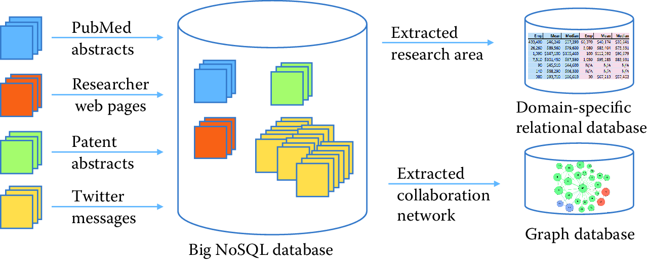
Figure 4.1: A research project may use a NoSQL database to accumulate large amounts of data from many different sources, and then extract selected subsets to a relational or other database for more structured processing
4.3 Relational DBMSs
We now provide a more detailed description of relational DBMSs. Relational DBMSs implement the relational data model, in which data are represented as sets of records organized in tables. This model is particularly well suited for the structured data with which we frequently deal in the social sciences; we discuss in Section NoSQL databases alternative data models, such as those used in NoSQL databases.
We use the data shown in Figure 4.2 to introduce key concepts. These two CSV format files describe grants made by the US National Science Foundation (NSF). One file contains information about grants, the other information about investigators. How should you proceed to manipulate and analyze these data?
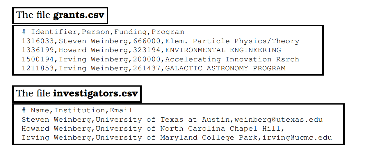
Figure 4.2: CSV files representing grants and investigators. Each line in the first table specifies a grant number, investigator name, total funding amount, and NSF program name; each line in the second gives an investigator name, institution name, and investigator email address
The main concept underlying the relational data model is a table (also referred to as a relation): a set of rows (also referred to as tuples, records, or observations), each with the same columns (also referred to as fields, attributes or variables). A database consists of multiple tables. For example, we show in Figure 4.3 how the data contained in the two CSV files of Figure 4.2 may be represented as two tables. The Grants table contains one tuple for each row in grants.csv, with columns GrantID, Person, Funding, and Program. The table contains one tuple for each row in investigators.csv, with columns ID, Name, Institution, and Email. The CSV files and tables contain essentially the same information, albeit with important differences (the addition of an ID field in the Investigators table, the substitution of an ID column for the Person column in the Grants table) that we will explain below.
The use of the relational data model provides for physical independence: a given table can be stored in many different ways. SQL queries are sets of instructions to execute commands written in terms of the logical representation of tables (i.e., their schema definition). Consequently, even if the physical organization of the data changes (e.g., a different layout is used to store the data on disk, or a new index is created to speed up access for some queries), the queries need not change. Another advantage of the relational data model is that, since a table is a set, in a mathematical sense, simple and intuitive set operations (e.g., union, intersection) can be used to manipulate the data, as we discuss below. We can easily, for example, determine the intersection of two relations (e.g., grants that are awarded to a specific institution), as we describe in the following. The database further ensures that the data comply with the model (e.g., data types, key uniqueness, entity relationships), essentially providing core quality assurance.
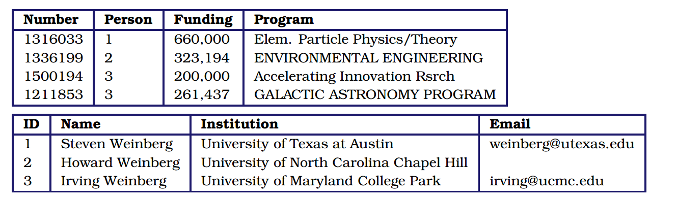
Figure 4.3: Relational tables Grants and Investigators corresponding to the grants.csv and investigators.csv data in Figure 4.2, respectively. The only differences are the representation in a tabular form, the introduction of a unique numerical investigator identifier (ID) in the Investigators table, and the substitution of that identifier for the investigator name in the Grants table
4.3.1 Structured Query Language (SQL)
We use query languages to manipulate data in a database (e.g., to add, update, or delete data elements) and to retrieve (raw and aggregated) data from a database (e.g., data elements that certain properties). Most Relational DBMSs support SQL, a simple, powerful query language with a strong formal foundation based on logic, a foundation that allows relational DBMSs to perform a wide variety of sophisticated optimizations. SQL is used for three main purposes:
Data definition: e.g., creation of new tables,
Data manipulation: queries and updates,
Control: creation of assertions to protect data integrity.
We introduce each of these features in the following, although not in that order, and certainly not completely. Our goal here is to give enough information to provide the reader with insights into how relational databases work and what they do well; an in-depth SQL tutorial is beyond the scope of this book, but we highly recommend checking the references at the end of this chapter.
4.3.2 Manipulating and querying data
SQL and other query languages used in DBMSs support the concise, declarative specification of complex queries. Because we are eager to show you something immediately useful, we cover these features first, before talking about how to define data models.
Example: Identifying grants of more than $200,000 Here is an SQL query to identify all grants with total funding of at most $200,000:
select * from Grants
where Funding <= 200,000;
Notice SQL’s declarative nature: this query can be read almost as the English language statement, “select all rows from the Grants table for which the Funding column has value less than or equal 200,000.” This query is evaluated as follows:
The input table specified by the
fromclause,Grants, is selected.The condition in the
whereclause,Funding <= 200,000, is checked against all rows in the input table to identify those rows that match.The
selectclause specifies which columns to keep from the matching rows, that is, which columns constitute the schema of the output table. (The “*” indicates that all columns should be kept.)
The answer, given the data in Figure 4.3, is the following single-row table. (The fact that an SQL query returns a table is important when it comes to creating more complex queries: the result of a query can be stored into the database as a new table, or passed to another query as input.)
| Number | Person | Funding | Program |
|---|---|---|---|
| 1500194 | 3 | 200,000 | Accelerating Innovation Rsrch |
DBMSs automatically optimize declarative queries such as the example that we just presented, translating them into a set of low-level data manipulations (an imperative query plan) that can be evaluated efficiently. This feature allows users to write queries without having to worry too much about performance issues—the database does the worrying for you. For example, a DBMS need not consider every row in the Grants table in order to identify those with funding less than $200,000, a strategy that would be slow if the Grants table were large: it can instead use an index to retrieve the relevant records much more quickly. We discuss indices in more detail in Section Database optimizations.
The querying component of SQL supports a wide variety of manipulations on tables, whether referred to explicitly by a table name (as in the example just shown) or constructed by another query. We just saw how to use the select operator to both pick certain rows (what is termed selection) and certain columns (what is called projection) from a table.
Example: Finding grants awarded to an investigator
We want to find all grants awarded to the investigator with name “Irving Weinberg.” The information required to answer this question is distributed over two tables, Grants and Investigators, and so we join the two tables to combine tuples from both:
select Number, Name, Funding, Program
from Grants, Investigators
where Grants.Person = Investigators.ID
and Name = "Irving Weinberg";
This query combines tuples from the Grants and Investigators tables for which the Person and ID fields match. It is evaluated in a similar fashion to the query presented above, except for the from clause: when multiple tables are listed, as here, the conditions in the where clause are checked for all different combinations of tuples from the tables defined in the from clause (i.e., the cartesian product of these tables)—in this case, a total of \(3\times 4 = 12\) combinations. We thus determine that Irving Weinberg has two grants. The query further selects the Number, Name, Funding, and Program fields from the result, giving the following:
| Number | Person | Funding | Program |
|---|---|---|---|
| 1500194 | Irving Weinberg | 200,000 | Accelerating Innovation Rsrch |
| 1211853 | Irving Weinberg | 261,437 | GALACTIC ASTRONOMY PROGRAM |
This ability to join two tables in a query is one example of how SQL permits concise specifications of complex computations. This joining of tables via a cartesian product operation is formally called a cross join. Other types of join are also supported. We describe one such, the inner join, in Section Spatial databases.
SQL aggregate functions allow for the computation of aggregate statistics over tables. For example, we can use the following query to determine the total number of grants and their total and average funding levels:
select count(*) as 'Number', sum(Funding) as 'Total',
       avg(Funding) as 'Average'
from Grants;
This yields the following:
| Number | Total | Average |
|---|---|---|
| 4 | 1444631 | 361158 |
The group by operator can be used in conjunction with the aggregate functions to group the result set by one or more columns. For example, we can use the following query to create a table with three columns: investigator name, the number of grants associated with the investigator, and the aggregate funding:
select Name, count(*) as 'Number',
       avg(Funding) as 'Average funding'
from Grants, Investigators
where Grants.Person = Investigators.ID
group by Name;
We obtain the following:
| Name | Number | Average Funding |
|---|---|---|
| Steven Weinberg | 1 | 666000 |
| Howard Weinberg | 1 | 323194 |
| Irving Weinberg | 2 | 230719 |
4.3.3 Schema design and definition
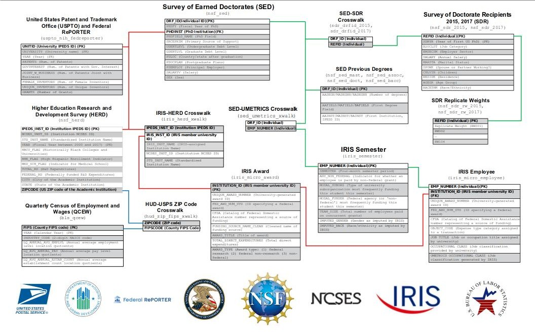
Figure 4.4: A database schema can show the ways in which many tables are linked. Here, there are individual-links (shown in green) as well as institution-level links (shown in red) and location-level links (shown in blue).
When using a pre-existing database, you will be given the database design that includes tables, rows, and columns. But, when you are starting with your own data and need to create a database, the first step is to come up with the design of the database.
We have seen that a relational database comprises a set of tables. The task of specifying the structure of the data to be stored in a database is called logical design. This task may be performed by a database administrator, in the case of a database to be shared by many people, or directly by users, if they are creating databases themselves. More specifically, the logical design process involves defining a schema. A schema comprises a set of tables (including, for each table, its columns and their types), their relationships, and integrity constraints.
The first step in the logical design process is to identify the entities that need to be modeled. In our example, we identified two important classes of entity: “grants” and “investigators.” We thus define a table for each; each row in these two tables will correspond to a unique grant or investigator, respectively. (In a more complete and realistic design, we would likely also identify other entities, such as institutions and research products.) During this step, we will often find ourselves breaking information up into multiple tables, so as to avoid duplicating information.
For example, imagine that we were provided grant information in the form of one CSV file rather than two, with each line providing a grant number, investigator, funding, program, institution, and email. In this file, the name, institution, and email address for Irving Weinberg would then appear twice, as he has two grants, which can lead to errors when updating values and make it difficult to represent certain information. (For example, if we want to add an investigator who does not yet have a grant, we will need to create a tuple (row) with empty slots for all columns (variables) associated with grants.) Thus we would want to break up the single big table into the two tables that we defined here. This breaking up of information across different tables to avoid repetition of information is referred to as normalization.3031
The second step in the design process is to define the columns that are to be associated with each entity. For each table, we define a set of columns. For example, given the data in Figure 4.2, the grant table should include columns for award identifier, title, investigator, and award amount; for an investigator, the columns will be name, university, and email address. In general, we will want to ensure that each row in our table has a key: a set of columns that uniquely identifies that row. In our example tables, grants are uniquely identified by Number and investigators by ID.
The third step in the design process is to capture relationships between entities. In our example, we are concerned with just one relationship, namely that between grants and investigators: each grant has an investigator. We represent this relationship between tables by introducing a Person column in the Grants table, as shown in Figure 4.3. Note that we do not simply duplicate the investigator names in the two tables, as was the case in the two CSV files shown in Figure 4.2: these names might not be unique, and the duplication of data across tables can lead to later inconsistencies if a name is updated in one table but not the other.
The final step in the design process is to represent integrity constraints (or rules) that must hold for the data. In our example, we may want to specify that each grant must be awarded to an investigator; that each value of the grant identifier column must be unique (i.e., there cannot be two grants with the same number); and that total funding can never be negative. Such restrictions can be achieved by specifying appropriate constraints at the time of schema creation, as we show in Listing Grantdata, which contains the code used to create the two tables that make up our schema.
Listing Grantdata contains four SQL statements. The first two statements, lines 1 and 2, simply set up our new database. The create table statement in lines 1 and 2 creates our first table. It specifies the table name (Investigators) and, for each of the four columns, the column name and its type.32 Relational DBMSs offer a rich set of types to choose from when designing a table: for example, int or integer (synonyms); real or float(synonyms); char(n), a fixed-length string of n characters; and varchar(n), a variable-length string of up to n characters. Types are important for several reasons. First, they allow for more efficient encoding of data. For example, the Funding field in the grants.csv file of Figure 4.2 could be represented as a string in the Grants table, char(15), say, to allow for large grants. By representing it as a floating point number instead (line 15 in Listing Grantdata), we reduce the space requirement per grant to just four bytes. Second, types allow for integrity checks on data as they are added to the database: for example, that same type declaration for Funding ensures that only valid numbers will be entered into the database. Third, types allow for type-specific operations on data, such as arithmetic operations on numbers (e.g., min, max, sum).
Other SQL features allow for the specification of additional constraints on the values that can be placed in the corresponding column. For example, the not null constraints for Name and Institution (lines 6, 7) indicate that each investigator must have a name and an institution, respectively. (The lack of such a constraint on the Email column shows that an investigator need not have an email address.)
create database grantdata;
use grantdata;

create table Investigators (
    ID int auto_increment,
    Name varchar(100) not null,
    Institution varchar(256) not null,
    Email varchar(100),
    primary key(ID)
);

create table Grants (
    Number int not null,
    Person int not null,
    Funding float unsigned not null,
    Program varchar(100),
    primary key(Number)
);4.3.4 Loading data
So far we have created a database and two empty tables. The next step is to add data to the tables. We can of course do that manually, row by row, but in most cases we will import data from another source, such as a CSV file. Listing Load data shows the two statements that load the data of Figure 4.2 into our two tables. (Here and elsewhere in this chapter, we use the MySQL DBMS. The SQL syntax used by different DBMSs differs in various, mostly minor ways.) Each statement specifies the name of the file from which data is to be read and the table into which it is to be loaded. The fields terminated by "," statement tells SQL that values are separated by columns, and ignore 1 lines tells SQL to skip the header. The list of column names is used to specify how values from the file are to be assigned to columns in the table.
For the Investigators table, the three values in each row of the investigators.csv file are assigned to the Name, Institution, and Email columns of the corresponding database row. Importantly, the auto_increment declaration on the ID column (line 5 in Listing Grantdata) causes values for this column to be assigned automatically by the DBMS, as rows are created, starting at 1. This feature allows us to assign a unique integer identifier to each investigator as its data are loaded.
load data local infile "investigators.csv"
    into table Investigators
    fields terminated by ","
    ignore 1 lines
    (Name, Institution, Email);

load data local infile "grants.csv" into table Grants
    fields terminated by ","
    ignore 1 lines
    (Number, @var, Funding, Program)
set Person = (select ID from Investigators
where Investigators.Name=@var);For the Grants table, the load data call (lines 7–12) is somewhat more complex. Rather than loading the investigator name (the second column of each line in our data file, represented here by the variable @var) directly into the database, we use an SQL query (the select statement in lines 11–12) to retrieve from the Investigators table the ID corresponding to that name. By thus replacing the investigator name with the unique investigator identifier, we avoid replicating the name across the two tables.
4.3.5 Transactions and crash recovery
A DBMS protects the data that it stores from computer crashes: if your computer stops running suddenly (e.g., your operating system crashes or you unplug the power), the contents of your database are not corrupted. It does so by supporting transactions. A transaction is an atomic sequence of database actions. In general, every SQL statement is executed as a transaction. You can also specify sets of statements to be combined into a single transaction, but we do not cover that capability here. The DBMS ensures that each transaction is executed completely even in the case of failure or error: if the transaction succeeds, the results of all operations are recorded permanently (“persisted”) in the database, and if it fails, all operations are “rolled back” and no changes are committed. For example, suppose we ran the following SQL statement to convert the funding amounts in the table from dollars to euros, by scaling each number by 0.9. The update statement specifies the table to be updated and the operation to be performed, which in this case is to update the Funding column of each row. The DBMS will ensure that either no rows are altered or all are altered.
update Grants set Grants.Funding = Grants.Funding*0.9;Transactions are also key to supporting multi-user access. The concurrency control mechanisms in a DBMS allow multiple users to operate on a database concurrently, as if they were the only users of the system: transactions from multiple users can be interleaved to ensure fast response times, while the DBMS ensures that the database remains consistent. While entire books could be (and have been) written on concurrency in databases, the key point is that read operations can proceed concurrently, while update operations are typically serialized.
4.3.6 Database optimizations
A relational DBMS applies query planning and optimization methods with the goal of evaluating queries as efficiently as possible. For example, if a query asks for rows that fit two conditions, one cheap to evaluate and one expensive, a relational DBMS may filter first on the basis of the first condition, and then apply the second conditions only to the rows identified by that first filter. These sorts of optimization are what distinguish SQL from other programming languages, as they allow the user to write queries declaratively and rely on the DBMS to come up with an efficient execution strategy.
Nevertheless, the user can help the DBMS to improve performance. The single most powerful performance improvement tool is the index, an internal data structure that the DBMS maintains to speed up queries. While various types of indices can be created, with different characteristics, the basic idea is simple. Consider the column in our table. Assume that there are \(N\) rows in the table. In the absence of an index, a query that refers to a column value (e.g., where ID=3) would require a linear scan of the table, taking on average \(N/2\) comparisons and in the worst case \(N\) comparisons. A binary tree index allows the desired value to be found with just \(\log_2 N\) comparisons.
Example: Using indices to improve database performance
Consider the following query:
select ID, Name, sum(Funding) as TotalFunding
  from Grants, Investigators
    where Investigators.ID=Grants.Person
  group by ID;
This query joins our two tables to link investigators with the grants that they hold, groups grants by investigator (using group by), and finally sums the funding associated with the grants held by each investigator. The result is the following:
| ID | Name | TotalFunding |
|---|---|---|
| 1 | Steven Weinberg | 666000 |
| 2 | Howard Weinberg | 323194 |
| 3 | Irving Weinberg | 230719 |
In the absence of indices, the DBMS must compare each row in Investigators with each row in Grants, checking for each pair whether Investigators.ID = Grants.Person holds. As the two tables in our sample database have only three and four rows, respectively, the total number of comparisons is only \(3\times 4=12\). But if we had, say, 1 million investigators and 1 million grants, then the DBMS would have to perform 1 trillion comparisons, which would take a long time. (More importantly, it would have to perform a large number of disk I/O operations, if the tables did not fit in memory.) An index on the ID column of the Investigators table reduces the number of operations dramatically, as the DBMS can then take each of the 1 million rows in the Grants table and, for each row, identify the matching row(s) in Investigators via an index lookup rather than a linear scan.
In our example table, the ID column has been specified to be a primary key, and thus an index is created for it automatically. If it were not, we could easily create the desired index as follows:
alter table Investigators add index(ID);It can be difficult for the user to determine when an index is required. A good rule of thumb is to create an index for any column that is queried often, that is, appears on the right-hand side of a where statement that is to be evaluated frequently. However, the presence of indices makes updates more expensive, as every change to a column value requires that the index be rebuilt to reflect the change. Thus, if your data are highly dynamic, you should carefully select which indices to create. (For bulk load operations, a common practice is to drop indices prior to the data import, and re-create them once the load is completed.) Also, indices take disk space, so you need to consider the tradeoff between query efficiency and resources.
The explain command can be useful for determining when indices are required. For example, we show in the following some of the output produced when we apply explain to our query. (For this example, we have expanded the two tables to 1,000 rows each, as our original tables are too small for MySQL to consider the use of indices.) The output provides useful information such as the key(s) that could be used, if indices exist (Person in the Grants table, and the primary key, ID, for the Investigators table); the key(s) that are actually used (the primary key, ID, in the Investigators table); the column(s) that are compared to the index (Investigators.ID is compared with Grants.Person); and the number of rows that must be considered (each of the 1,000 rows in Grants is compared with one row in Investigators, for a total of 1,000 comparisons).
mysql> explain select ID, Name, sum(Funding) as TotalFunding
       from Grants, Investigators
       where Investigators.ID=Grants.Person group by ID;

+---------------+---------------+---------+---------------+------+
| table         | possible_keys | key     | ref           | rows |
+---------------+---------------+---------+---------------+------+
| Grants        | Person        | NULL    | NULL          | 1000 |
| Investigators | PRIMARY       | PRIMARY | Grants.Person |    1 |
+---------------+---------------+---------+---------------+------+
Contrast this output with the output obtained for equivalent tables in which is not a primary key. In this case, no keys are used and thus \(1{,}000\times 1{,}000=1{,}000{,}000\) comparisons, and the associated disk reads, must be performed.
+---------------+---------------+------+------+------+
| table         | possible_keys | key  | ref  | rows |
+---------------+---------------+------+------+------+
| Grants        | Person        | NULL | NULL | 1000 |
| Investigators | ID            | NULL | NULL | 1000 |
+---------------+---------------+------+------+------+
A second way in which the user can contribute to performance improvement is by using appropriate table definitions and data types. Most DBMSs store data on disk. Data must be read from disk into memory before it can be manipulated. Memory accesses are fast, but loading data into memory is expensive: accesses to main memory can be a million times faster than accesses to disk. Therefore, to ensure queries are efficient, it is important to minimize the number of disk accesses. A relational DBMS automatically optimizes queries: based on how the data are stored, it transforms a SQL query into a query plan that can be executed efficiently, and chooses an execution strategy that minimizes disk accesses. But users can contribute to making queries efficient. As discussed above, the choice of types made when defining schemas can make a big difference. As a rule of thumb, only use as much space as needed for your data: the smaller your records, the more records can be transferred to main memory using a single disk access. The design of relational tables is also important. If you put all columns in a single table (i.e., you do not normalize), more data may come into memory than is required.
4.3.7 Caveats and challenges
It is important to keep the following caveats and challenges in mind when using SQL technology with social science data.
Data cleaning
Data created outside an SQL database, such as data in files, are not always subject to strict constraints: data types may not be correct or consistent (e.g., numeric data stored as text) and consistency or integrity may not be enforced (e.g., absence of primary keys, missing foreign keys). Indeed, as the reader probably knows well from experience, data are rarely perfect. As a result, the data may fail to comply with strict SQL schema requirements and fail to load, in which case either data must be cleaned before or during loading, or the SQL schema must be relaxed.
Missing values
Care must be taken when loading data in which some values may be missing or blank. SQL engines represent and refer to a missing or blank value as the built-in constant null. Counterintuitively, when loading data from text files (e.g., CSV), many SQL engines require that missing values be represented explicitly by the term null; if a data value is simply omitted, it may fail to load or be incorrectly represented, for example as zero or the empty string ("") instead of null. Thus, for example, the second row in the investigators.csv file of Figure 4.2:
Howard Weinberg,University of North Carolina Chapel Hill,
may need to be rewritten as:
Howard Weinberg,University of North Carolina Chapel Hill,null
Metadata for categorical variables
SQL engines are metadata poor: they do not allow extra information to be stored about a variable (field) beyond its base name and type (int, char, etc., as introduced in Section Schema design and definition). They cannot, for example, record directly the fact that the column class can only take one of three values, animal, vegetable, or mineral, or what these values mean. Common practice is thus to store information about possible values in another table (commonly referred to as a dimension table) that can be used as a lookup and constraint, as in the following:
| Value | Description |
|---|---|
animal |
Is alive |
vegetable |
Grows |
mineral |
Isn’t alive and doesn’t grow |
A related concept is that a column or list of columns may be declared primary key or unique. Such a statement specifies that no two tuples of the table may agree in the specified column—or, if a list if columns is provided, in all of those columns. There can be only one primary key for a table, but several unique columns. No column of a primary key can ever be null in any tuple. But columns declared unique may have nulls, and there may be several tuples with null.
4.4 Linking DBMSs and other tools
Query languages such as SQL are not general-purpose programming languages; they support easy, efficient access to large data sets, are extremely efficient for specific types of analysis, but may not be the right choice for all analysis. When complex computations are required, one can embed query language statements into a programming language or statistical package. For example, we might want to calculate the interquartile range of funding for all grants. While this calculation can be accomplished in SQL, the resulting SQL code will be complicated (depending on which flavor of SQL your database supports). Languages like Python make such statistical calculations straightforward, so it is natural to write a Python (or R, SAS, Stata, etc.) program that connects to the DBMS that contains our data, fetches the required data from the DBMS, and then calculates the interquartile range of those data. The program can then, if desired, store the result of this calculation back into the database.
Many relational DBMSs also have built-in analytical functions or often now support different programming languages, providing significant in-database statistical and analytical capabilities and alleviating the need for external processing.
from mysql.connector import MySQLConnection, Error
from python_mysql_dbconfig import read_db_config

def retrieve_and_analyze_data():
    try:
        # Open connection to the MySQL database
        dbconfig = read_db_config()
        conn = MySQLConnection(**dbconfig)
        cursor = conn.cursor()
        # Transmit the SQL query to the database
        cursor.execute('select Funding from Grants;')
        # Fetch all rows of the query response
        rows = [row for row in cur.fetchall()]
        calculate_inter_quartile_range(rows)
    except Error as e:
        print(e)
    finally:
        cursor.close()
        conn.close()

if __name__ == '__main__':
retrieve_and_analyze_data()Example: Embedding database queries in Python
The Python script in Listing Embedding shows how this embedding of database queries in Python is done. This script establishes a connection to the database, transmits the desired SQL query to the database (line 7–9), retrieves the query results into a Python array (line 11), and calls a Python procedure (not given) to perform the desired computation (line 14). A similar program could be used to load the results of a Python (or R, SAS, Stata, etc.) computation into a database.
Example: Loading other structured data
We saw in Listing Load data how to load data from CSV files into SQL tables. Data in other formats, such as the commonly used JSON, can also be loaded into a relational DBMS. Consider, for example, the following JSON format data, a simplified version of data shown in Chapter Working with Web Data and APIs.
[
  {
    institute : Janelia Campus,
    name : Laurence Abbott,
    role : Senior Fellow,
    state : VA,
    town : Ashburn
  },
  {
    institute : Jackson Lab,
    name : Susan Ackerman,
    role : Investigator,
    state : ME,
    town : Bar Harbor
  }
]
While some relational DBMSs (such as PostgresQL) provide built-in support for JSON objects, we assume here that we want to convert these data into normal SQL tables. Using one of the many utilities for converting JSON into CSV, we can construct the following CSV file, which we can load into an SQL table using the method shown earlier.
institute,name,role,state,town
Janelia Campus,Laurence Abbott,Senior Fellow,VA,Ashburn
Jackson Lab,Susan Ackerman,Investigator,ME,Bar Harbor
But into what table? The two records each combine information about a person with information about an institute. Following the schema design rules given in Section Schema design and definition, we should normalize the data by reorganizing them into two tables, one describing people and one describing institutes. Similar problems arise when JSON documents contain nested structures. For example, consider the following alternative JSON representation of the data above. Here, the need for normalization is yet more apparent.
[
  {
    name : Laurence Abbott,
    role : Senior Fellow,
    employer : { institute : Janelia Campus,
                 state : VA,
                 town : Ashburn}
  },
  {
    name : Susan Ackerman,
    role : Investigator,
    employer: { institute : Jackson Lab,
                state : ME,
                town : Bar Harbor}
  }
]
Thus, the loading of JSON data into a relational database usually requires both work on schema design (Section Schema design and definition) and data preparation.
4.5 NoSQL databases
While relational DBMSs have dominated the database world for several decades, other database technologies exist and indeed have become popular for various classes of applications in recent years. As we will see, these alternative technologies have typically been motivated by a desire to scale the quantities of data and/or number of users that can be supported, and/or to support specialized data types (e.g., unstructured data, graphs). Here we review some of these alternatives and the factors that may motivate their use.
4.5.1 Challenges of scale: The CAP theorem
For many years, the big relational database vendors (Oracle, IBM, Sybase, Microsoft) have been the mainstay of how data were stored. During the Internet boom, startups looking for low-cost alternatives to commercial relational DBMSs turned to MySQL and PostgreSQL. However, these systems proved inadequate for big websites as they could not cope well with large traffic spikes, for example when many customers all suddenly wanted to order the same item. That is, they did not scale.
An obvious solution to scaling databases is to partition data across multiple computers, for example by distributing different tables, or different rows from the same table, over multiple computers. We may also want to replicate popular data, by placing copies on more than one computer. However, partitioning and replication also introduce challenges, as we now explain. Let us first define some terms. In a system that comprises of multiple computers:
Consistency indicates that all computers see the same data at the same time.
Availability indicates that every request receives a response about whether it succeeded or failed.
Partition tolerance indicates that the system continues to operate even if a network failure prevents computers from communicating.
An important result in distributed systems (the so-called “CAP theorem”, Brewer (2012)) observes that it is not possible to create a distributed system with all three properties. This situation creates a challenge with large transactional data sets. Partitioning and replication needed in order to achieve high performance, but as the number of computers grows, so too does the likelihood of network disruption among pair(s) of computers. A network disruption can prevent some replicas of a data item from being updated, compromising consistency. As strict consistency cannot be achieved at the same time as availability and partition tolerance, the DBMS designer must choose between high consistency and high availability for a particular system.
The right combination of availability and consistency will depend on the needs of the service. For example, in an e-commerce setting, it makes sense to choose high availability for a checkout process, in order to ensure that requests to add items to a shopping cart (a revenue-producing process) can be honored. Errors can be hidden from the customer and sorted out later. However, for order submission—when a customer submits an order—it makes sense to favor consistency because several services (credit card processing, shipping and handling, reporting) need to access the data simultaneously. However, in almost all cases, availability is chosen over consistency.
4.5.2 NoSQL and key–value stores
Relational DBMSs were traditionally motivated by the need for transaction processing and analysis, which led them to put a premium on consistency and availability. This led the designers of these systems to provide a set of properties summarized by the acronym ACID (Gray 1981; Silberschatz, Korth, and Sudarshan 2010):
Atomic: All work in a transaction completes (i.e., is committed to stable storage) or none of it completes.
Consistent: A transaction transforms the database from one consistent state to another consistent state.
Isolated: The results of any changes made during a transaction are not visible until the transaction has committed.
Durable: The results of a committed transaction survive failures.
The need to support extremely large quantities of data and numbers of concurrent clients has led to the development of a range of alternative database technologies that relax consistency and thus these ACID properties in order to increase scalability and/or availability. These systems are commonly referred to as NoSQL (for “not SQL”—or, more recently, “not only SQL,” to communicate that they may support SQL-like query languages) because they usually do not require a fixed table schema nor support joins and other SQL features. Such systems are sometimes referred to as BASE (Fox et al. 1997): Basically Available (the system seems to work all the time), Soft state (it does not have to be consistent all the time), and Eventually consistent (it becomes consistent at some later time). The data systems used in essentially all large Internet companies (Google, Yahoo!, Facebook, Amazon, eBay) are BASE.
Dozens of different NoSQL DBMSs exist, with widely varying characteristics as summarized in Table 4.2. The simplest are key–value stores such as Redis, Amazon Dynamo, Apache Cassandra, and Project Voldemort. We can think of a key–value store as a relational database with a single table that has just two columns, key and value, and that supports just two operations: store (or update) a key–value pair, and retrieve the value for a given key.
Example: Representing investigator data in a NoSQL database We might represent the contents of the investigators.csv file of Figure 4.2 (in a NoSQL database) as follows.
| Key | Value |
|---|---|
| Investigator_StevenWeinberg_Institution | University of Texas at Austin |
| Investigator_StevenWeinberg_Email | [email protected] |
| Investigator_HowardWeinberg_Institution | University of North Carolina Chapel Hill |
| Investigator_IrvingWeinberg_Institution | University of Maryland College Park |
| Investigator_IrvingWeinberg_Email | [email protected] |
A client can then read and write the value associated with a given key by using operations such as the following:
Get(key) returns the value associated with key.
Put(key, value) associates the supplied value with key.
Delete(key) removes the entry for key from the data store.
Key–value stores are thus particularly easy to use. Furthermore, because there is no schema, there are no constraints on what values can be associated with a key. This lack of constraints can be useful if we want to store arbitrary data. For example, it is trivial to add the following records to a key–value store; adding this information to a relational table would require schema modifications.
| Key | Value |
|---|---|
| Investigator_StevenWeinberg_FavoriteColor | Blue |
| Investigator_StevenWeinberg_Awards | Nobel |
Another advantage is that if a given key would have no value (e.g., Investigator_HowardWeinberg_Email), we need not create a record. Thus, a key–value store can achieve a more compact representation of sparse data, which would have many empty fields if expressed in relational form.
A third advantage of the key–value approach is that a key–value store is easily partitioned and thus can scale to extremely large sizes. A key–value DBMS can partition the space of keys (e.g., via a hash on the key) across different computers for scalability. It can also replicate key–value pairs across multiple computers for availability. Adding, updating, or querying a key–value pair requires simply sending an appropriate message to the computer(s) that hold that pair.
The key–value approach also has disadvantages. As we can see from the example, users must be careful in their choice of keys if they are to avoid name collisions. The lack of schema and constraints can also make it hard to detect erroneous keys and values. Key–value stores typically do not support join operations (e.g., “which investigators have the Nobel and live in Texas?”). Many key–value stores also relax consistency constraints and do not provide transactional semantics.
4.5.3 Other NoSQL databases
The simple structure of key–value stores allows for extremely fast and scalable implementations. However, as we have seen, many interesting data cannot be easily modeled as key–value pairs. Such concerns have motivated the development of a variety of other NoSQL systems that offer, for example, richer data models: document-based (CouchDB and MongoDB), graph-based (Neo4J) and column-based (Cassandra, HBase) databases, and graph databases.
In document-based databases, the value associated with a key can be a structured document: for example, a JSON document, permitting the following representation of our investigators.csv file plus the additional information that we just introduced.
| Key | Value |
|---|---|
| Investigator_StevenWeinberg | { institution : University of Texas at Austin, email : [email protected], favcolor : Blue, award : Nobel } |
| Investigator_HowardWeinberg | { institution : University of North Carolina Chapel Hill } |
| Investigator_IrvingWeinberg | { institution : University of Maryland College Park, email : [email protected] } |
Associated query languages may permit queries within the document, such as regular expression searches, and retrieval of selected fields, providing a form of a relational DBMS’s selection and projection capabilities (Section Manipulating and querying data). For example, MongoDB allows us to ask for documents in a collection called that have “University of Texas at Austin” as their institution and the Nobel as an award.
db.investigators.find( { institution: 'University of Texas at Austin', award: 'Nobel' } )
A column-oriented DBMS stores data tables by columns rather than by rows, as is common practice in relational DBMSs. This approach has advantages in settings where aggregates must frequently be computed over many similar data items: for example, in clinical data analysis. Google Cloud BigTable and Amazon RedShift are two cloud-hosted column-oriented NoSQL databases. HBase and Cassandra are two open source systems with similar characteristics. (Confusingly, the term column oriented is also often used to refer to SQL database engines that store data in columns instead of rows: for example, Google BigQuery, HP Vertica, Terradata, and the open source MonetDB. Such systems are not to be confused with column-based NoSQL databases.)
Graph databases store information about graph structures in terms of nodes, edges that connect nodes, and attributes of nodes and edges. Proponents argue that they permit particularly straightforward navigation of such graphs, as when answering queries such as “find all the friends of the friends of my friends”—a task that would require multiple joins in a relational database.
4.6 Spatial databases
Social science research commonly involves spatial data. Socioeconomic data may be associated with census tracts, data about the distribution of research funding and associated jobs with cities and states, and crime reports with specific geographic locations. Furthermore, the quantity and diversity of such spatially resolved data are growing rapidly, as are the scale and sophistication of the systems that provide access to these data. For example, just one urban data store, Plenario, contains many hundreds of data sets about the city of Chicago (Catlett et al. 2014).
Researchers who work with spatial data need methods for representing those data and then for performing various queries against them. Does crime correlate with weather? Does federal spending on research spur innovation within the locales where research occurs? These and many other questions require the ability to quickly determine such things as which points exist within which regions, the areas of regions, and the distance between two points. Spatial databases address these and many other related requirements.
Example: Spatial extensions to relational databases
Spatial extensions have been developed for many relational databases: for example, Oracle Spatial, DB2 Spatial, and SQL Server Spatial. We use the PostGIS extensions to the PostgreSQL relational database here. These extensions implement support for spatial data types such as point, line, and polygon, and operations such as st_within (returns true if one object is contained within another), st_dwithin (returns true if two objects are within a specified distance of each other), and st_distance (returns the distance between two objects). Thus, for example, given two tables with rows for schools and hospitals in Illinois (illinois_schools and illinois_hospitals, respectively; in each case, the column the_geom is a polygon for the object in question) and a third table with a single row representing the city of Chicago (chicago_citylimits), we can easily find the names of all schools within the Chicago city limits:
select illinois_schools.name
  from illinois_schools, chicago_citylimits
  where st_within(illinois_schools.the_geom,
                  chicago_citylimits.the_geom);
We join the two tables and , with the constraint constraining the selected rows to those representing schools within the city limits. Here we use the inner join introduced in Section Manipulating and querying data. This query could also be written as:
select illinois_schools.name
  from illinois_schools left join chicago_citylimits
  on st_within(illinois_schools.the_geom,
                  chicago_citylimits.the_geom);
We can also determine the names of all schools that do not have a hospital within 3,000 meters:
select s.name as 'School Name'
    from illinois_schools as s
        left join illinois_hospitals as h
          on st_dwithin(s.the_geom, h.the_geom, 3000)
    where h.gid is null;
Here, we use an alternative form of the join operator, the left join—or, more precisely, the left excluding join. The expression
table1 left join table2 on constraint
returns all rows from the left table (table1) with the matching rows in the right table (table2), with the result being null in the right side when there is no match. This selection is illustrated in the middle column of Figure 4.5. The addition of the where h.gid is null then selects only those rows in the left table with no right-hand match, as illustrated in the right-hand column of Figure 4.5. Note also the use of the as operator to rename the columns illinois_schools and illinois_hospitals. In this case, we rename them simply to make our query more compact.
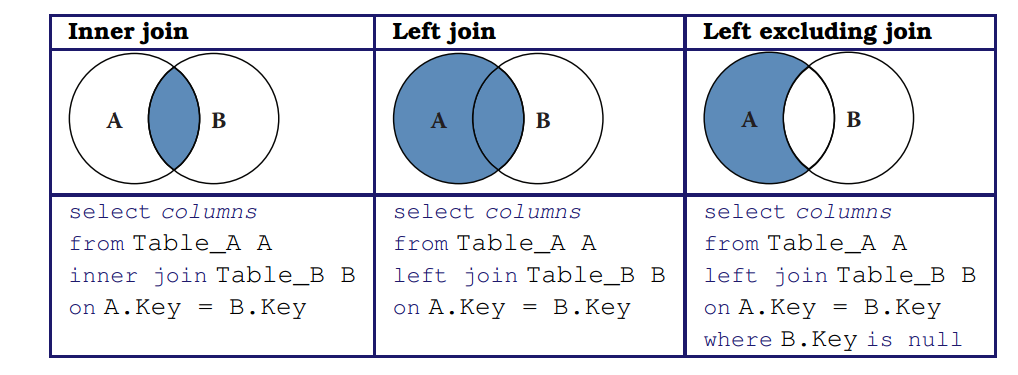
Figure 4.5: Three types of join illustrated: the inner join, the left join, and left excluding join
4.7 Which database to use?
The question of which DBMS to use for a social science project depends on many factors. We introduced some relevant rules in Table 4.1. We expand on those considerations here.
4.7.1 Relational DBMSs
If your data are structured into rows and columns, then a relational DBMS is almost certainly the right technology to use. Many open source, commercial, and cloud-hosted relational DBMSs exist. Among the open source DBMSs, MySQL and PostgreSQL (often simply called Postgres) are particularly widely used. MySQL is the most popular. It is particularly easy to install and use, but does not support all features of the SQL standard. PostgreSQL is fully standard compliant and supports useful features such as full text search and the PostGIS extensions mentioned in the previous section. We recommend you start with Postgres.
Popular commercial relational DBMSs include Microsoft SQL Server, Oracle, IBM DB2, Teradata, and Sybase. These systems are heavily used in commercial settings. There are free community editions, and some large science projects use enterprise features via licensing: for example, the Sloan Digital Sky Survey uses Microsoft SQL Server (Szalay et al. 2002) and the CERN high-energy physics lab uses Oracle (Girone 2008).
We also see increasing use being made of cloud-hosted relational DBMSs such as Amazon Relational Database Service (RDS; this supports MySQL, PostgreSQL, and various commercial DBMSs), Microsoft Azure, and Google Cloud SQL. These systems obviate the need to install local software, administer a DBMS, or acquire hardware to run and scale your database. Particularly if your database is bigger than can fit on your workstation, a cloud-hosted solution can be a good choice, both for scalability but also for ease of configuration and management.
4.7.2 NoSQL DBMSs
Some social science problems have the scale that might motivate the use of a NoSQL DBMS. Furthermore, while defining and enforcing a schema can involve some effort, the benefits of so doing are considerable. Thus, the use of a relational DBMS is usually to be recommended.
Nevertheless, as noted in Section DBMS: When and why, there are occasions when a NoSQL DBMS can be a highly effective, such as when working with large quantities of unstructured data. For example, researchers analyzing large collections of Twitter messages frequently store the messages in a NoSQL document-oriented database such as MongoDB. NoSQL databases are also often used to organize large numbers of records from many different sources, as illustrated in Figure 4.1.
4.8 Summary
A key message of this book is that you should, whenever possible, use a database. Database management systems are one of the great achievements of information technology, permitting large amounts of data to be stored and organized so as to allow rapid and reliable exploration and analysis. They have become a central component of a great variety of applications, from handling transactions in financial systems to serving data published in websites. They are particularly well suited for organizing social science data and for supporting analytics for data exploration.
DBMSs provide an environment that greatly simplifies data management and manipulation. They make many easy things trivial, and many hard things easy. They automate many other error-prone, manual tasks associated with query optimization. While they can by daunting to those unfamiliar with their concepts and workings, they are in fact easy to use. A basic understanding of databases and of when and how to use DBMSs is an important element of the social data scientist’s knowledge base.
4.9 Resources
The enormous popularity of DBMSs means that there are many good books to be found. Classic textbooks such as those by Silberschatz et al. (2010) and Ramakrishnan and Gherke (2002) provide a great deal of technical detail. The DB Engines website collects information on DBMSs.33 There are also many useful online tutorials, and of course StackExchange and other online forums often have answers to your technical questions.
Turning to specific technologies, the SQL Cookbook (Molinaro 2005) provides a wonderful introduction to SQL. We also recommend the SQL Cheatsheet34 and a useful visual depiction of different SQL join operators (Moffatt 1999). Two good books on the PostGIS geospatial extensions to the PostgreSQL database are the PostGIS Cookbook (Corti et al. 2014) and PostGIS in Action (Obe and Hsu 2015). The online documentation is also excellent.35 The monograph NoSQL Databases (Strauch 2009) provides much useful technical detail.
We did not consider in this chapter the native extensible Markup Language (XML) and Resource Description Framework (RDF) triple stores, as these are not typically used for data management. However, they do play a fundamental role in metadata and knowledge management. See, for example, Sesame (Broekstra, Kampman, and Van Harmelen 2002).36
If you are interested in the state of database and data management research, the relatively recent Beckman Report (Abadi et al. 2014) provides a useful perspective.
The Databases notebook of Chapter Workbooks provides an introduction to working with SQL.37
References
Abadi, Daniel, Rakesh Agrawal, Anastasia Ailamaki, Magdalena Balazinska, Philip A Bernstein, Michael J Carey, Surajit Chaudhuri, et al. 2014. “The Beckman Report on Database Research.” ACM SIGMOD Record 43 (3). ACM: 61–70.
Brewer, Eric. 2012. “CAP Twelve Years Later: How the ‘Rules’ Have Changed.” Computer 45 (2). IEEE: 23–29.
Broekstra, Jeen, Arjohn Kampman, and Frank Van Harmelen. 2002. “Sesame: A Generic Architecture for Storing and Querying RDF and RDF Schema.” In The Semantic Web—ISWC 2002, 54–68. Springer.
Catlett, Charlie, Tanu Malik, Brett Goldstein, Jonathan Giuffrida, Yetong Shao, Alessandro Panella, Derek Eder, et al. 2014. “Plenario: An Open Data Discovery and Exploration Platform for Urban Science.” Bulletin of the IEEE Computer Society Technical Committee on Data Engineering 37: 27–42.
Corti, Paolo, Thomas J. Kraft, Stephen Vincent Mather, and Bborie Park. 2014. PostGIS Cookbook. Packt Publishing.
Fox, Armando, Steven D. Gribble, Yatin Chawathe, Eric A. Brewer, and Paul Gauthier. 1997. “Cluster-Based Scalable Network Services.” ACM SIGOPS Operating Systems Review 31 (5). ACM.
Girone, Maria. 2008. “CERN Database Services for the LHC Computing Grid.” In Journal of Physics: Conference Series. Vol. 119. 5. IOP Publishing.
Gray, Jim. 1981. “The Transaction Concept: Virtues and Limitations.” In Proceedings of the Seventh International Conference on Very Large Data Bases, 7:144–54.
Kohler, Ulrich, and Frauke Kreuter. 2012. Data Analysis Using Stata. 3rd Edition. Stata Press.
Moffatt, C. L. 1999. “Visual Representation of SQL Joins.” http://www.codeproject.com/Articles/33052/Visual-Representation-of-SQL-Joins.
Molinaro, Anthony. 2005. SQL Cookbook: Query Solutions and Techniques for Database Developers. O’Reilly Media.
Obe, Regina O., and Leo S. Hsu. 2015. PostGIS in Action, 2nd Edition. Manning Publications.
Ramakrishnan, Raghu, and Johannes Gehrke. 2002. Database Management Systems, 3rd Edition. McGraw-Hill.
Silberschatz, Abraham, Henry F. Korth, and S. Sudarshan. 2010. Database System Concepts, 6th Edition. McGraw-Hill.
Strauch, Christof. 2009. “NoSQL Databases.” http://www.christof-strauch.de/nosqldbs.pdf.
Szalay, Alexander S., Jim Gray, Ani R. Thakar, Peter Z. Kunszt, Tanu Malik, Jordan Raddick, Christopher Stoughton, and Jan vandenBerg. 2002. “The SDSS Skyserver: Public Access to the Sloan Digital Sky Server Data.” In Proceedings of the 2002 Acm Sigmod International Conference on Management of Data, 570–81. ACM.
A scripting language is a programming language used to automate tasks that could otherwise be performed one by one by the user.↩
For example, the Panel Study of Income Dynamics (http://psidonline.isr.umich.edu) has a series of files that are related and can be combined through common identifier variables (Institute for Social Research 2013).↩
DBMS is a system that interacts with users, other applications, and the database itself to capture and analyze data.↩
Some key DBMS features are often lacking in standard statistical packages: a standard query language (with commands that allow analyses or data manipulation on a subgroup of cases defined during the analysis, for example “group by …,” “order by …”), keys (for speed improvement), and an explicit model of a relational data structure.↩
Sometimes, as discussed in Chapter Record Linkage, the links are one to one and sometimes one to many.↩
A schema defines the structure of a database in a formal language defined by the DBMS. See Section Schema design and definition.↩
Normalization involves organizing columns and tables of a relational database to minimize data redundancy.↩
Normalization can be done in statistical packages as well. For example, as noted above, PSID splits its data into different files linked through ID variables. The difference here is that the DBMS makes creating, navigating, and querying the resulting data particularly easy.↩
These storage types will be familiar to many of you from statistical software packages.↩