Chapter 11 Bias and Fairness
Kit T. Rodolfa, Pedro Saleiro, and Rayid Ghani
Interest in algorithmic fairness and bias has been growing recently (for good reason), but it’s easy to get lost in the large number of definitions and metrics. There are many different, often competing, ways to measure whether a given model is statistically “fair” but it’s important to remember to start from the social and policy goals for equity and fairness and map those to the statistical properties we want in our models to help achieve those goals. In this chapter, we provide an overview of these statistical metrics along with some concrete examples to help navigate these concepts and understand the trade-offs involved in choosing to optimize to one metric over others, focusing on the metrics relevant to binary classification methods used frequently in risk-based models for policy settings.
11.1 Introduction
In Chapter Machine Learning, you learned about several of the concepts, tools, and approaches used in the field of machine learning and how they can be applied in the social sciences. In that chapter, we focused on evaluation metrics such as precision (positive predictive value), recall (sensitivity), area-under-curve (AUC), and accuracy, that are often used to measure the performance of machine learning methods. In most (if not all) public policy problems, a key goal for the analytical systems being developed is to help achieve equitable outcomes for society and we need to understand how to design systems that lead to equity.
When machine learning models are being used to make decisions, they cannot be separated from the social and ethical context in which they are applied, and those developing and deploying these models must take care to do so in a manner that accounts for both accuracy and fairness. In this chapter, we will discuss sources of potential bias in the modeling pipeline, as well as some of the ways that bias introduced by a model can be measured, with a particular focus on classification problems. Unfortunately, just as there is no single machine learning algorithm that is best suited to every application, no one fairness metric will fit every situation. However, we hope this chapter will provide you with a grounding in the available ways of measuring algorithmic fairness that will help you navigate the trade-offs involved putting these into practice in your own applications.
11.2 Sources of Bias
Bias may be introduced into a machine learning project at any step along the way and it is important to carefully think through each potential source and how it may affect your results. In many cases, some sources may be difficult to measure precisely (or even at all), but this doesn’t mean these potential biases can be readily ignored when developing interventions or performing analyses.
11.2.1 Sample Bias
You’re likely familiar with sampling issues as a potential source of bias in the contexts of causal inference and external validity in the social science literature. A biased sample can be just as problematic for machine learning as it can be for inference, and predictions made on individuals or groups not represented in the training set are likely to be unreliable. As such, any application of machine learning should start with a careful understanding of data generating process for the training and test sets. What is the relevant population for the project and how might some individuals be incorrectly excluded or included from the data available for modeling or analysis?
If there is a mismatch between the available training data and the population to whom the model will be applied, you may want to consider whether it is possible to collect more representative data. A model to evaluate the risk of health violations at restaurants may be of limited applicability if the only training data available is based on inspections that resulted from reported complaints. In such a case, an initial trial of randomized inspections might provide a more representative dataset. However, this may not always be possible. For instance, in the case of bail determinations, labeled data will only be available for individuals who are released under the existing system.
How does the available training data relate to the population that the model will be applied to? If there is a mismatch here, is it possible to collect more appropriate data? In the example of bail determination, for instance, you only have subsequent outcome data for individuals who were actually released in the past and lack the counterfactual/potential outcomes for those who were detained.
Even if the training data matches the population, are their underlying systemic biases involved in defining that population in general? For instance, over-policing of black neighborhoods might mean the population of incarcerated individuals is unrepresentative of the population of individuals who have committed a given crime and even a representative sample of the jail population might not be the appropriate universe for a given policy or social science question.
For data with a time component or models that will be deployed to aid future decisions, are there relevant policy changes in the past that may make data from certain periods of time less relevant? Pending policy changes going forward that may affect the modeling population?
Measurement here might be difficult, but it is nevertheless helpful to think through each of these questions in detail. Often, other sources of data (even in aggregate form) can provide some insight on how representative your data may be, including census data, surveys, and academic studies in the relevant area.
11.2.2 Label (Outcome) Bias
Regardless of whether your dataset reflects a representative sample of the relevant population for your intervention or analysis, there may also be bias inherent in the labels (that is, the measured outcomes) associated with individuals in that data.
One mechanism by which bias may be introduced is in how the label/outcome itself is defined. For instance, a study of recidivism might use a new arrest as an outcome variable when it really cares about committing a new crime. However, if some groups are policed more heavily than others, using arrests to define the outcome variable may introduce bias into the system’s decisions. Similarly, a label that relies on the number of days an individual has been incarcerated would reflect known biases in sentence lengths between black and white defendants.
A related mechanism is measurement error. Even when the outcome of interest is well-defined and can be measured directly, bias may be introduced through differential measurement accuracy across groups. For instance, data collected through survey research might suffer from language barriers or cultural differences in social desirability that introduce measurement errors across groups.
11.2.3 Machine Learning Pipeline Bias
Biases can be introduced by the handling and transformation of data throughout the machine learning pipeline as well, requiring careful consideration as you ingest data, create features, and model outcomes of interest. Below are a few examples at each stage of the process, but these are far from exhaustive and intended only to help motivate thinking about how bias might be introduced in your own projects.
**Ingesting Data:** The process of loading, cleaning, and reconciling data from a variety of data sources (often referred to as ETL) can introduce a number of errors that might have differential downstream impacts on different populations:
Are your processes for matching individuals across data sources equally accurate across different populations? For instance, married vs maiden names may bias match rates against women, while inconsistencies in handling of multi-part last names may make matching less reliable for hispanic individuals.
Nickname dictionaries used in record reconciliation might be derived from different populations than your population of interest.
A data loading process that drops records with “special characters” might inadvertently exclude names with accents or tildes.
Feature Engineering: Biases are easy to introduce during the process of constructing features, both in the handling of features that relate directly to protected classes as well as information that correlates with these populations (such as geolocation). A few examples include:
Dictionaries to infer age or gender from name might be derived from a population that is not relevant to your problem.
Handling of missing values and combining “other” categories can become problematic, especially for multi-racial individuals or people with non-binary gender.
Thought should be given to how race and ethnicity indicators are collected – are these self-reported, recorded by a third party, or inferred from other data? The data collection process may inform the accuracy of the data and how errors differ across populations.
Features that rely on geocoding to incorporate information based on distances or geographic aggregates may miss homeless individuals or provide less predictive power for more mobile populations.
Modeling: The model itself may introduce bias into decisions made from its scores by performing worse on some groups relative to others (many examples have been highlighted in popular press recently, such as racial biases in facial recognition algorithms and gender biases in targeting algorithms for job advertisement on social media). Because of the complex correlation structure of the data, it generally isn’t sufficient to simply leave out the protected attributes and assume this will result in fair outcomes. Rather model performance across groups needs to be measured directly in order to understand and address any biases. However, there are many (often incompatible) ways to define fairness and Section metrics will take a closer look at these options in much more detail.
Much of the remainder of this chapter focuses on how we might define and measure fairness at the level of the machine learning pipeline itself. In Section metrics, we will introduce several of the metrics used to measure algorithmic fairness and in Section applications we discuss how these can be used in the process of evaluating and selecting machine learning models.
11.2.4 Application Bias
A final potential source of bias worth considering is how the model or analysis might be put into use in practice. One way this might happen is through heterogeneity in the effectiveness of an intervention across groups. For instance, imagine a machine learning model to identify individuals most at risk for developing diabetes in the next 3 years for a particular preventive treatment. If the treatment is much more effective for individuals with a certain genetic background relative to others, the overall outcome of the effort might be to exacerbate disparities in diabetes rates even if the model itself is modeling risk in an unbiased way.
Likewise, it is important to be aware of the risk of discriminatory applications of a machine learning model. Perhaps a model developed to screen out unqualified job candidates is only “trusted” by a hiring manager for female candidates but often ignored or overridden for men. In a perverse way, applying an unbiased model in such a context might serve to increase inequities by giving bad actors more information with which to (wrongly) justify their discriminatory practices.
While there may be relatively little you can do to detect or mitigate these types of bias at the modeling stage, performing a trial to compare current practice with a deployed model can be instructive where doing so is feasible. Keep in mind, of course, that the potential for machine learning systems to be applied in biased ways shouldn’t be construed as an argument against developing these systems at all any more than it would be reasonable to suggest that current practices are likely to be free of bias. Rather, it is an argument for thinking carefully about both the status quo and how it may change in the presence of such a system, putting in place legal and technical safeguards to help ensure that these methods are applied in socially responsible ways.
11.2.5 Considering Bias When Deploying Your Model
Ultimately, what we care about is some global idea of how putting a model into practice will affect some overall concept of social welfare and fairness influenced by all of these possible sources of bias. While this is generally impossible to measure in a quantitative way, it can provide a valuable framework for qualitatively evaluating the potential impact of your model. For most of the remainder of this chapter, we consider a set of more quantitative metrics that can be applied to the predictions of a machine learning pipeline specifically, but it is important to keep in mind that these metrics only apply to the sample and labels you have and ignoring other sources of bias that may be at play in the underlying data generating process could result in unfair outcomes even when applying a model that appears to be “fair” by your chosen metric.
11.3 Dealing with Bias
11.3.1 Define Bias
Section bias examples provided some examples for how bias might be introduced in the process of using machine learning to work with a dataset. While far from exhaustive as a source of potential bias in an overall application, these biases can be more readily measured and addressed through choices made during data preparation, modeling, and model selection. This section focuses on detecting and understanding biases introduced at this stage of the process.
One key challenge, however, is that there is no universally-accepted definition of what it means for a model to be fair. Take the example of a model being used to make bail determinations. Different people might consider it “fair” if:
It makes mistakes about denying bail to an equal number of white and black individuals
The chances that a given black or white person will be wrongly denied bail is equal, regardless of race
Among the jailed population, the probability of having been wrongly denied bail is independent of race
For people who should be released, the chances that a given black or white person will be denied bail is equal
In different contexts, reasonable arguments can be made for each of these potential definitions, but unfortunately, not all of them can hold at the same time. The remainder of this section explores these competing options and how to approach them in more detail.
11.3.2 Definitions
Most of the metrics used to assess model fairness relate either to the types of errors a model might make or how predictive the model is across different groups. For binary classification models (which we focus on here), these are generally derived from values in the confusion matrix (see Figure 7.9 and Chapter Machine Learning for more details):
True Positives (\(TP\)) are individuals for whom both the model prediction and actual outcome are positive labels.
False Positives (\(FP\)) are individuals for whom both the model predicts a positive label, but the actual outcome is a negative label.
True Negatives (\(TN\)) are individuals for whom both the model prediction and actual outcome are negative labels.
False Negatives (\(FN\)) are individuals for whom both the model predicts a negative label, but the actual outcome is a positive label.
Based on these four categories, we can calculate several ratios that are instructive for thinking about the equity of a model’s predictions in different situations (Sections punitive example and assistive example provide some detailed examples here):
False Positive Rate (\(FPR\)) is the fraction of individuals with negative actual labels who the model misclassifies with a positive predicted label.90
False Negative Rate (\(FNR\)) is the fraction of individuals with positive actual labels who the model misclassifies with a negative predicted label.91
False Discovery Rate (\(FDR\)) is the fraction of individuals who the model predicts to have a positive label but for whom the actual label is negative.92
False Omission Rate (\(FOR\)) is the fraction of individuals who the model predicts to have a negative label but for whom the actual label is positive.93
Precision is the fraction of individuals who the model predicts to have a positive label about whom this prediction is correct.94
Recall is the fraction of individuals with positive actual labels who the model has correctly classified as such.95
For the first two metrics (\(FPR\) and \(FNR\)), notice that the denominator is based on actual outcomes (rather than model predictions), while in the next two (\(FDR\) and \(FOR\)) the denominator is based on model predictions (whether an individual falls above or below the threshold used to turn model scores into 0/1 predicted classes). The final two metrics relate to correct predictions rather than errors, but are directly related to error measurements (that is, \(\textrm{recall} = 1-FNR\) and \(\textrm{precision} = 1-FDR\)) and may sometimes have better properties for calculating model bias.
Notice that the metrics defined here require the use of a threshold to turn modeled scores into 0/1 predicted classes and are therefore most useful when either a threshold is well-defined for the problem (e.g., when available resources mean a program can only serve a given number of individuals) or where calculating these metrics at different threshold levels might be used (along with model performance metrics) to choose a threshold for application. In some cases, it may also be of interest to think about equity across the full distribution of the modeled score (Chouldechova 2017; Kleinberg, Mullainathan, and Raghavan 2017). Common practices in these situations are to look at how model performance metrics such as the area under the receiver-operator curve (\(AUC-ROC\)) or model calibration compared across subgroups (such as by race, gender, age). Or, in cases where the underlying causal relationships are well-known, counterfactual methods (Kilbertus et al. 2017; Kusner et al. 2017) may also be used to assess a model’s bias (these methods may also be useful when you suspect label bias to be an issue in your data). We don’t explore these topics deeply here, but refer you out to the relevant references if you would like to learn more.
11.3.3 Choosing Bias Metrics
Any of the metrics defined above can be used to calculate disparities across groups in your data and (unless you have a perfect model) many of them cannot be balanced across subgroups at the same time. As a result, one of the most important — and frequently most challenging — aspects of measuring bias in your machine learning pipeline is simply understanding how “fairness” should be defined for your particular case.
In general, this requires consideration of the project’s goals and a detailed discussion between the data scientists, decision makers, and those who will be affected by the application of the model. Each perspective may have a different concept of fairness and a different understanding of harm involved in making different types of errors, both at individual and societal levels. Importantly, data scientists have an critical role in this conversation, both as the experts in understanding how different concepts of fairness might translate into metrics and measurement and as individuals with experience deploying similar models. While there is no universally correct definition of fairness, nor one that can be learned from the data, this doesn’t excuse the data scientists from responsibility for taking part in the conversation around fairness and equity in their models and helping decision makers understand the options and trade-offs involved.
Practically speaking, coming to an agreement on how fairness should be measured in a purely abstract manner is likely to be difficult. Often it can be instructive instead to explore different options and metrics based on preliminary results, providing tangible context for potential trade-offs between overall performance and different definitions of equity and helping guide stakeholders through the process of deciding what to optimize. The remainder of this section looks at some of the metrics that may be of particular interest in different types of applications:
If your intervention is punitive in nature (e.g., determining whom to deny bail), individuals may be harmed by intervening on them in error so you may care more about metrics that focus on false positives. Section punitive example provides an example to guide you through what some of these metrics mean in this case.
If your intervention is assistive in nature (e.g., determining who should receive a food subsidy), individuals may be harmed by failing to intervene on them when they have need, so you may care more about metrics that focus on false negatives Section assistive example provides an example to guide you through metrics that may be applicable in this case.
If your resources are significantly constrained such that you can only intervene on a small fraction of the population at need, some of the metrics described here may be of limited use and Section constrained assistive describes this case in more detail.
Navigating the many options for defining bias in a given context is a difficult and nuanced process, even for those familiar with the underlying statistical concepts. In order to help facilitate these conversations between data scientists and stakeholders, we developed the Fairness Tree depicted in Figure 11.1. While it certainly can’t provide a single “right” answer for a given context, our hope is that the Fairness Tree can act as a tool to help structure the process of arriving at an appropriate metric (or set of metrics) to focus on.
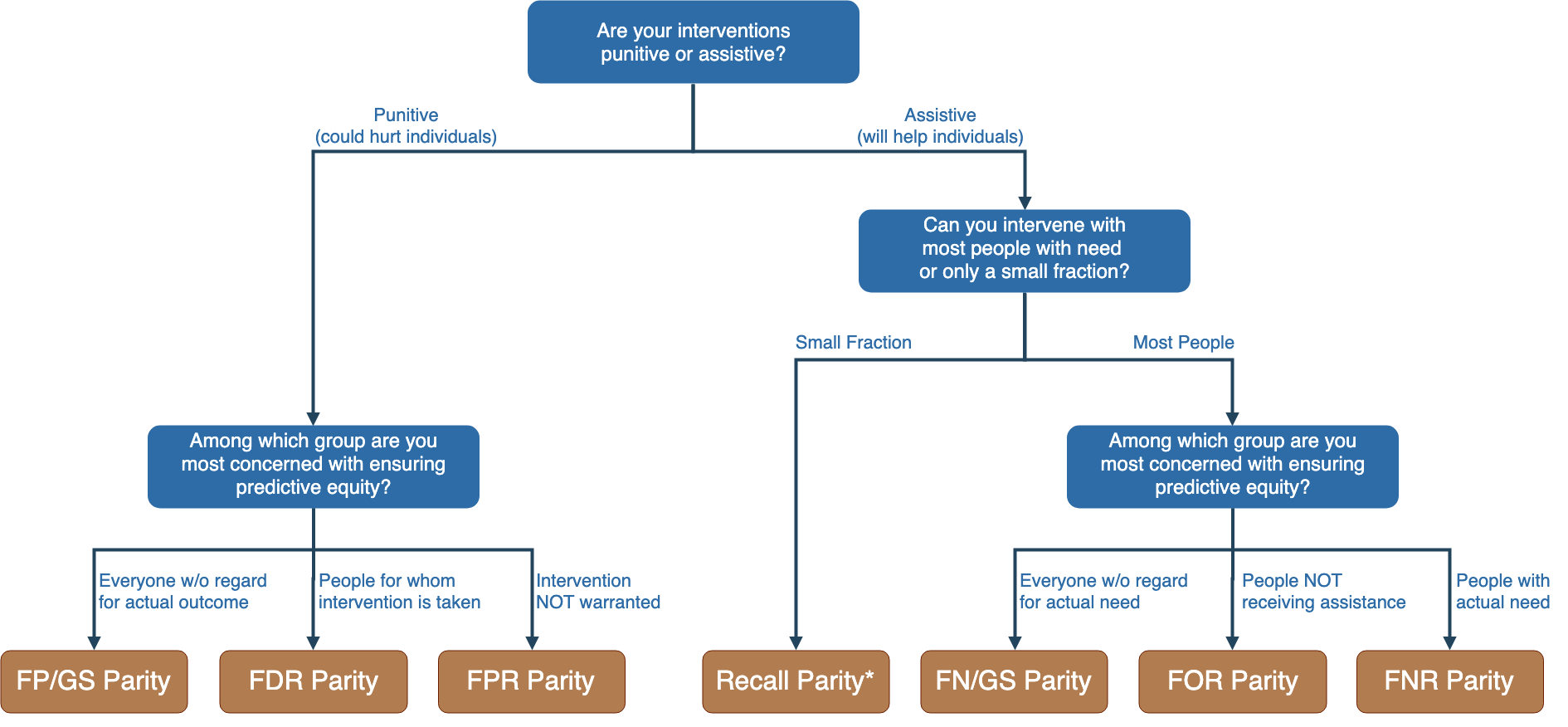
Figure 11.1: Fairness Tree
11.3.4 Punitive Example
When the application of a risk model is punitive in nature, individuals may be harmed by being incorrectly included in the “high risk” population that receives an intervention. In an extreme case, we can think of this as incorrectly detaining an innocent person in jail. Hence, with punitive interventions, we focus on bias and fairness metrics based on false positives.
11.3.4.1 Count of False Positives
We might naturally think about the number of people wrongly jailed from each group as reasonable place to start for assessing whether our model is biased. Here, we are concerned with statements like “twice as many people from Group A were wrongly convicted as from Group B.”
In probabilistic terms, we could express this as: \[P(\textrm{wrongly jailed, group $i$}) = C~~~\forall~i\] Where \(C\) is a constant value. Or, alternatively, \[\frac{FP_i}{FP_j} = 1~~~\forall~i,j\] Where \(FP_i\) is the number of false positives in group \(i\).
However, it is unclear whether differences in the number of false positives across groups reflect unfairness in the model. For instance, if there are twice as many people in Group A as there are in Group B, some might deem the the situation described above as fair from the standpoint that the composition of the false positives reflects the composition of the groups. This brings us to our second metric:
11.3.4.2 Group Size-Adjusted False Positives
By accounting for differently sized groups, we ask the question, “just by virtue of the fact that an individual is a member of a given group, what are the chances they’ll be wrongly convicted?”
In terms of probability, \[P(\textrm{wrongly jailed $\mid$ group $i$}) = C~~~\forall~i\] Where \(C\) is a constant value. Or, alternatively, \[\frac{FP_i}{FP_j} = \frac{n_i}{n_j}~~~\forall~i,j\] Where \(FP_i\) is the number of false positives and \(n_i\) the total number of individuals in group \(i\).
While this metric might feel like it meets a reasonable criteria of avoiding treating groups differently in terms of classification errors, there are other sources of disparities we might care about as well. For instance, suppose there are 10,000 individuals in Group A and 30,000 in Group B. Suppose further that 100 individuals from each group are jail, with 10 Group A people wrongly convicted and 30 Group B people wrongly convicted. We’ve balanced the number of false positives by group size (0.1% for both groups) so there are no disparities as far as this metric is concerned, but note that 10% of the jailed Group A individuals are innocent compared to 30% of the jailed Group B individuals. The next metric is concerned with unfairness in this way:
11.3.4.3 False Discovery Rate
The False Discovery Rate (\(FDR\)) focuses specifically on the people who are affected by the intervention—in the example above, among the 200 people in jail, what are the group-level disparities in rates of wrong convictions. The jail example is particularly instructive here as we could imagine the social cost of disparities manifesting directly through inmates observing how frequently different groups are wrongly convicted.
In probabilistic terms, \[P(\textrm{wrongly jailed $\mid$ jailed, group $i$}) = C~~~\forall~i\] Where \(C\) is a constant value. Or, alternatively, \[\frac{FP_i}{FP_j} = \frac{k_i}{k_j}~~~\forall~i,j\] Where \(FP_i\) is the number of false positives and \(k_i\) the total number of jailed individuals in group \(i\).
11.3.4.4 False Positive Rate
The False Positive Rate (\(FPR\)) focuses on a different subset, specifically, the individuals who should not be subject to the intervention. Here, this would ask, “for an innocent person, what are the chances they will be wrongly convicted by virtue of the fact that they’re a member of a given group?”
In probabilistic terms, \[P(\textrm{wrongly jailed $\mid$ innocent, group $i$}) = C~~~\forall~i\] Where \(C\) is a constant value. Or, alternatively, \[\frac{FP_i}{FP_j} = \frac{n_i \times (1-p_i)}{n_j \times (1-p_j)}~~~\forall~i,j\] Where \(FP_i\) is the number of false positives, \(n_i\) the total number of individuals, and \(p_i\) is the prevalence (here, rate of being truly guilty) in group \(i\).
The difference between the choosing to focus on the \(FPR\) and group size-adjusted false positives is somewhat nuanced and warrants highlighting:
Having no disparities in group size-adjusted false positives implies that, if I were to choose a random person from a given group (regardless of group-level crime rates or their individual guilt or innocence), I would have the same chance of picking out a wrongly convicted person across groups.
Having no disparities in \(FPR\) implies that, if I were to choose a random innocent person from a given group, I would have the same chance of picking out a wrongly convicted person across groups.
11.3.4.5 Trade-Offs in Metric Choice
By way of example, imagine you have a society with two groups (A and B) and a criminal process with equal \(FDR\) and group-size adjusted false positives with:
Group A has 1000 total individuals, of whom 100 have been jailed with 10 wrongfully convicted. Suppose the other 900 are all guilty.
Group B has 3000 total individuals, of whom 300 have been jailed with 30 wrongfully convicted. Suppose the other 2700 are all innocent.
In this case, \[\begin{aligned} &\frac{FP_A}{n_A} = \frac{10}{1000} = 1.0\% \\ &FDR_A = \frac{10}{100} = 10.0\% \\ &FPR_A = \frac{10}{10} = 100.0\%\end{aligned}\]
while, \[\begin{aligned} &\frac{FP_B}{n_B} = \frac{30}{3000} = 1.0\% \\ &FDR_B = \frac{30}{300} = 10.0\% \\ &FPR_B = \frac{30}{2730} = 1.1\%\end{aligned}\]
That is,
A randomly chosen individual has the same chance (1.0%) of being wrongly convicted regardless of which group they belong to
In both groups, a randomly chosen person who is in jail has the same chance (10.0%) of actually being innocent
HOWEVER, an innocent person in Group A is certain to be wrongly convicted, nearly 100 times the rate of an innocent person in Group B
While this is an exaggerated case for illustrative purposes, there is a more general principle at play here, namely: when prevalences differ across groups, disparities cannot be eliminated from both the \(FPR\) and group-size adjusted false positives at the same time (in the absence of perfect prediction).
While there is no universal rule for choosing a bias metric (or set of metrics) to prioritize, it is important to keep in mind that there are both theoretical and practical limits on the degree to which these metrics can be jointly optimized.
Balancing these trade-offs will generally require some degree of subjective judgment on the part of policy makers and should reflect both societal values arrived at with the input of those impacted by model-assisted decisions as well as practical constraints. For instance, if there is uncertainty in the quality of the labels (e.g., how well can we truly measure the size of the innocent population?), it may make more sense in practical terms to focus on the group-size adjusted false positives than \(FPR\).
11.3.5 Assistive Example
By contrast to the punitive case, when the application of a risk model is assistive in nature, individuals may be harmed by being incorrectly excluded from the “high risk” population that receives an intervention. Here, we use identifying families to receive a food assistance benefit as a motivating example. Where the punitive case focused on errors of inclusion through false positives, most of the metrics of interest in the assistive case focus on analogues that measure errors of omission through false negatives.
11.3.5.1 Count of False Negatives
A natural starting point for understanding whether a program is being applied fairly is to count how many people it is missing from each group, focusing on statements like “twice as many families with need for food assistance from Group A were missed by the benefit as from Group B.”
In probabilistic terms, we could express this as: \[P(\textrm{missed by benefit, group $i$}) = C~~~\forall~i\] Where \(C\) is a constant value. Or, alternatively, \[\frac{FN_i}{FN_j} = 1~~~\forall~i,j\] Where \(FN_i\) is the number of false negatives in group \(i\).
Differences in the number of false negatives by group, however, may be relatively limited in measuring equity when the groups are very different in size. If there are twice as many families in Group A as in Group B in the example above, the larger number of false negatives might not be seen as inequitable, which motivates our next metric:
11.3.5.2 Group Size-Adjusted False Negatives
To account for differently sized groups, one way of phrasing the question of fairness is to ask, “just by virtue of the fact that an individual is a member of a given group, what are the chances they will be missed by the food subsidy?”
That is, in terms of probability, \[P(\textrm{missed by benefit $\mid$ group $i$}) = C~~~\forall~i\] Where \(C\) is a constant value. Or, alternatively, \[\frac{FN_i}{FN_j} = \frac{n_i}{n_j}~~~\forall~i,j\] Where \(FN_i\) is the number of false negatives and \(n_i\) the total number of families in group \(i\).
While avoiding disparities on this metric focuses on the reasonable goal of treating different groups similarly in terms of classification errors, we may also want to directly consider two subsets within each group: (1) the set of families not receiving the subsidy, and (2) the set of families who would benefit from receiving the subsidy. We take a closer look at each of these cases below.
11.3.5.3 False Omission Rate
The False Omission Rate (\(FOR\)) focuses specifically on people on whom the program doesn’t intervene – in our example, the set of families not receiving the food subsidy. Such families will either be true negatives (that is, those not in need of the assistance) or false negatives (that is, those who did need assistance but were missed by the program), and the \(FOR\) asks what fraction of this set fall into the latter category.
In probabilistic terms, \[P(\textrm{missed by program $\mid$ no subsidy, group $i$}) = C~~~\forall~i\] Where \(C\) is a constant value. Or, alternatively, \[\frac{FN_i}{FN_j} = \frac{n_i-k_i}{n_j-k_j}~~~\forall~i,j\] Where \(FN_i\) is the number of false negatives, \(k_i\) the number of families receiving the subsidy, and \(n_i\) is the total number of families in group \(i\).
In practice, the \(FOR\) can be a useful metric in many situations, particularly because need can often be more easily measured among individuals not receiving a benefit than among those who do (for instance, when the benefit affects the outcome on which need is measured). However, when resources are constrained such that a program can only reach a relatively small fraction of the population, its utility is more limited. See constrained assistive for more details on this case.
11.3.5.4 False Negative Rate
The False Negative Rate (\(FNR\)) focuses instead on the set of people with need for the intervention. In our example, this asks the question, “for a family that needs food assistance, what are the chances they will be missed by the subsidy by virtue of the fact they’re a member of a given group?”
In probabilistic terms, \[P(\textrm{missed by subsidy $\mid$ need assistance, group $i$}) = C~~~\forall~i\] Where \(C\) is a constant value. Or, alternatively, \[\frac{FN_i}{FN_j} = \frac{n_i \times p_i}{n_j \times p_j}~~~\forall~i,j\] Where \(FN_i\) is the number of false negatives, \(n_i\) the total number of individuals, and \(p_i\) is the prevalence (here, rate of need for food assistance) in group \(i\).
As with the punitive case, there is some nuance in the difference between choosing to focus on group-size adjusted false negatives and the \(FNR\) that are worth pointing out:
Having no disparities in group size-adjusted false negatives implies that, if I were to choose a random family from a given group (regardless of group-level nutritional outcomes or their individual need), I would have the same chance of picking out a family missed by the program person across groups.
Having no disparities in \(FNR\) implies that, if I were to choose a random family with need for assistance from a given group, I would have the same chance of picking out one missed by the subsidy across groups.
Unfortunately, disparities in both of these metrics cannot be eliminated at the same time, except where the level of need is identical across groups or in the generally unrealist case of perfect prediction.
11.3.6 Special Case: Resource-Constrained Programs
In many real-world applications, programs may only have sufficient resources to serve a small fraction of individuals who might benefit. In these cases, some of the metrics described here may prove less useful. For instance, where the number of individuals served is much smaller than the number of individuals with need, the false omission rate will converge on the overall prevalence, and it will prove impossible to balance \(FOR\) across groups.
In such cases, group-level recall may provide a useful metric for thinking about equity, asking the question, “given that the program cannot serve everyone with need, is it at least serving different populations in a manner that reflects their level of need?”
In probabilistic terms, \[P(\textrm{received subsidy $\mid$ need assistance, group $i$}) = C~~~\forall~i\] Where \(C\) is a constant value. Or, alternatively, \[\frac{TP_i}{TP_j} = \frac{n_i \times p_i}{n_j \times p_j}~~~\forall~i,j\] Where \(TP_i\) is the number of true positives, \(n_i\) the total number of individuals, and \(p_i\) is the prevalence (here, rate of need for food assistance) in group \(i\).
Note that, unlike the metrics described above, using recall as an equity metric doesn’t explicitly focus on the mistakes being made by the program, but rather on how it is addressing need within each group. Nevertheless, balancing recall is equivalent to balancing the false negative rate across groups (note that \(recall = 1-FNR\)), but may be a more well-behaved metric for resource-constrained programs in practical terms. When the number of individuals served is small relative to need, \(FNR\) will approach 1 and ratios between group-level \(FNR\) values will not be particularly instructive, while ratios between group-level recall values will be meaningful.
As an aside, a focus on recall can also provide a lever that a program can use to consider options for achieving programmatic or social goals. For instance, if underlying differences in prevalence across groups is believed to be a result of social or historical inequities, a program may want to go further than balancing recall across groups, focusing even more heavily on historically under-served groups. One rule of thumb we have used in these cases is to balance recall relative to prevalence (however, there’s no theoretically “right” choice here and it’s generally best to consider a range of options):
\[\frac{recall_i}{recall_j} = \frac{p_i}{p_j}~~~\forall~i,j\]
The idea here is that (assuming the program is equally effective across groups), balancing recall will seek to improve outcomes at an equal rate across groups without impacting underlying disparities while a heavier focus on previously under-served groups might seek to both improve outcomes across groups while attempting to close these gaps as well.
11.4 Mitigating Bias
The metrics described in this chapter can be put to use in a variety of ways: auditing existing models and processes for equitable results, in the process of choosing a model to deploy, or in making choices about how a chosen model is put into use. This section provides some details about how you might approach each of these tasks.
11.4.1 Auditing Model Results
Because the metrics describe here rely only on the predicted and actual labels, no specific knowledge of the process by which the predicted labels are determined is needed to make use of them to assess bias and fairness in the results. Given this sort of labeled outcome data for any existing or proposed process (and our knowledge of how trustworthy the outcomes data may be) , bias audit tools such as Aequitas96 can be applied to help understand whether that process is yielding equitable results (for the various possible definitions of “equitable” described above).
Note that the existing process need not be a machine learning model: these equity metrics can be calculated for any set of decisions and outcomes, regardless of whether the decisions are derived from a model, judge, case worker, heuristic rule, or other process. And, in fact, it will generally be useful to make measures of equity in any existing processes which a model might augment or replace to help understand whether application of the model might improve, degrade, or leave unchanged the fairness of the existing system.
11.4.2 Model Selection
As described in Chapter Machine Learning, many different types of models (each in turn with many tune-able hyperparameters) can be brought to bear on a given machine learning problem, making the task of selecting a specific model to put into use an important step in the process of model development. Chapter Machine Learning described how this might be done by considering a model’s performance on various evaluation metrics, as well as how consistent that performance is across time or random splits of the data. This framework for model selection can naturally be extended to incorporate equity metrics, however doing so introduces a layer of complexity in determining how to evaluate trade-offs between overall performance and predictive equity.
Just as there is no one-size-fits-all metric for measuring equity that works in all contexts, you might choose to incorporate fairness in the model selection process in a variety of different ways. Here are a couple of options we have considered (though certainly not an exhaustive list):
If many models perform similarly on overall evaluation metrics of interest (say, above some reasonable threshold), how do they vary in terms of equitability?
How much “cost” in terms of performance do you have to pay to reach various levels of fairness? Think of this as creating a menu of options to explicitly show the trade-offs involved. For instance, imagine your best-performing model has a precision of 0.75 but FDR ratio of 1.3, but you can reach an FDR ratio of 1.2 by selecting a model with precision of 0.73, or a ratio of 1.1 at a precision of 0.70, or FDR parity at a precision of 0.64.
You may want to consider several of the equity metrics described above and might look at the model that performs best on each metric of interest (perhaps above some overall performance threshold) and consider choosing between these options.
If you are concerned about fairness across several subgroups (e.g., multiple categories of race/ethnicity, different age groups, etc), you might consider exploring the models that perform best for each subgroup in addition to those that perform similarly across groups
Another option might be to develop a single model selection parameter that penalizes performance by how far a model is from equity and explore how model choice changes based on how heavily you weight the equity parameter. Note, however, that when you are comparing equity across more than two groups, you will need to find a means of aggregating these to a single value (e.g., you might look at the average disparity, largest disparity, or use some weighting scheme to reflect different costs of disparities favoring different groups)
In most cases, this process will yield a number of options for a final model to deploy: some with better overall performance, some with better overall equity measures, and some with better performance for specific subgroups. Unlike model selection based on performance metrics alone, the final choice between these will generally involve a judgment call that reflects the project’s dual goals of balancing accuracy and equity. As such, the final choice of model from this narrowed menu of options is best treated as a discussion between the data scientists and stakeholders in the same manner as choosing how to define fairness in the first place.
11.4.3 Other Options for Mitigating Bias
Beyond incorporating measurements of equity into your model selection process, they can also inform how you put the model you choose into action. In general, disparities will vary as you vary the threshold used for turning continuous scores into 0/1 predicted classes. While many applications will dictate the total number of individuals who can be selected for intervention, it may still be useful to consider lower thresholds. For instance, in one project we saw large \(FDR\) disparities across age and race in our models when selecting the top 150 individuals for an intervention (a number dictated by programmatic capacity), but these disparities were mitigated by considering the top 1000 with relatively little cost in precision. This result suggested a strategy for deployment: use the model to select the 1000 highest risk individuals and randomly select 150 individuals from this set to stay within the program’s capacity while balancing equity and performance.
Another approach that can work well in some situations is to consider using different thresholds across groups to achieve more equitable results, which we explored in detail through a recent case study (Rodolfa et al. 2020). This is perhaps most robust where the metric of interest in monotonically increasing or decreasing with the number of individuals chosen for intervention (such as recall). This can be formulated in two ways:
For programs that have a target scale but may have some flexibility in budgeting, you can look at to what extent the overall size of the program would need to increase to achieve equitable results (or other fairness goals such as those described in constrained assistive. In this case, interventions don’t need to be denied to any individuals in the interest of fairness, but the program would incur some additional cost in order to achieve a more equitable result.
If the program’s scale is a hard constraint, you may still be able to use subgroup-specific thresholds to achieve more equitable results by selecting fewer of some groups and more of others relative to the single threshold. In this case, the program would not need additional costs of expansion, but some individuals who might have received the intervention based just on their score would need to be substituted for individuals with somewhat lower scores of under-represented subgroups.
As you’re thinking about equity in the application of your machine learning models, it’s also particularly important to keep in mind that measuring fairness in a model’s predictions is only a proxy for what you fundamentally care about: fairness in outcomes in the presence of the model. As a model is put into practice, you may find that the program itself is more effective for some groups than others, motivating either additional changes in your model selection process or customizing interventions to the specific needs of different populations (or individuals). Incorporating fairness into decisions about who is chosen to receive an intervention is an important first step, but shouldn’t be mistaken for a comprehensive solution to disparities in a program’s application and outcomes.
Some work is also being done investigating means for incorporating bias and fairness more directly in the process of model development itself. For instance, in may cases different numbers of examples across groups or unmeasured variables may contribute to a model having higher error rates on some populations than others and additional data collection (either more examples or new features) may help mitigate these biases where doing so is feasible (Chen, Johansson, and Sontag 2018). Other work is being done to explore the results of incorporating equity metrics directly into the loss functions used to train some classes of machine learning models, making balancing accuracy and equity an aspect of model training itself (Celis et al. 2019; Zafar et al. 2017). While we don’t explore these more advanced topics in depth here, we refer you to the cited articles for more detail.
11.5 Further Considerations
11.5.1 Compared to What?
While building machine learning models that are completely free of bias is an admirable goal, it may not always be an achievable one. Nevertheless, even an imperfect model may provide an improvement over current practices depending on the degree of bias involved in existing processes. It’s important to be cognizant of the existing context and make measurements of equity for current practices as well as new algorithms that might replace or augment them. The status quo shouldn’t be assumed to be free of bias because it is familiar any more than algorithms should be assumed capable of achieving perfection simply because they are complex. In practice, a more nuanced view is likely to yield better results: new models should be rigorously compared with current results and implemented when they are found to yield improvements but continually refined to improve on their outcomes over time as well.
11.5.2 Costs to Both Errors
In the examples in Section metrics, we focused on programs that could be considered purely assistive or purely punitive to illustrate some of the relevant metrics for such programs. While this classification may work for some real-world applications, in many others there will be costs associated with both errors of inclusion and errors of exclusion that need to be considered together in deciding both on how to think about fairness and how to put those definitions into practice through model selection and deployment. For the bail example, there are of course real costs to society both of jailing innocent people and releasing someone who does, in fact, commit a subsequent crime. In many programs where individuals may be harmed by being left out, errors of inclusion may mean wasted resources or even political backlash about excessive budgets.
In theory, you might imagine being able to assign some cost to each type of error — as well as to disparities in these errors across groups — and make a single, unified cost-benefit calculation of the net result of putting a given model into application in a given way. In practice, of course, making an even reasonable quantitative estimate of the individual and social costs of these different types of errors is likely infeasible in most cases. Instead, a more practical approach generally involves exploring a number of different options through different choices of models and parameters and using these options to motivate a conversation about the program’s goals, philosophy, and constraints.
11.5.3 What is the Relevant Population?
Related to the sample bias discussed in bias sources, understanding the relevant population for your machine learning problem is important both to the modeling itself and to your measures of equity. Calculation of metrics like the group-size adjusted false positive rate or false negative rate will vary depending on who is included in the denominator.
For instance, imagine modeling who should be selected to receive a given benefit using data from previous applicants and looking at racial equity based on these metrics. What population is actually relevant to thinking about equity in this case? It might be the pool of applicants available in your data, but it just as well might be the set of people who might apply if they had knowledge of the program (regardless of whether or not they actually do), or perhaps even the population at large (for instance, as measured by the census). Each of those choices could potentially lead to different conclusions about the fairness of the program’s decisions (either in the presence or absence of a machine learning model), highlighting the importance of understanding the relevant population and who might potentially be left out of your data as an element of how fairness is defined in your context. Keep in mind that determining (or at least making a reasonable estimate of) the correct population may at times require collecting additional data.
11.5.4 Continuous Outcomes
For the sake of simplicity, we focused here on binary classification problems to help illustrate the sorts of considerations you might encounter when thinking about fairness in the application of machine learning techniques. However, these considerations do of course extend to other types of problems, such as regression models of continuous outcomes.
In these cases, bias metrics can be formulated around aggregate functions of the errors a model makes on different types of individuals (such as the mean squared error and mean absolute error metrics you are likely familiar with from regression) or tests for similarity of the distributions of these errors across subgroups. Working with continuous outcomes adds an additional layer of complexity in terms of defining fairness to account for the magnitude of the errors being made (e.g., how do you choose between a model that makes very large errors on a small number of individuals vs one that makes relatively small errors on a large number of individuals?).
Unfortunately, the literature on bias and fairness in machine learning problems in other contexts (such as regression with continuous outcomes) is less rich than the work focused on classification, but if you would like to learn more about what has been done in this regard, we suggest consulting (Chouldechova and Roth 2018) for a good starting point (see, in particular, Section 3.5 of their discussion).
11.5.5 Considerations for Ongoing Measurement
The role of a data scientist is far from over when their machine learning model gets put into production. Making use of these models requires ongoing curation, both to guard against degradation in terms of performance or fairness as well as to constantly improve outcomes. The vast majority of models you put into production will make mistakes, and a responsible data scientist will seek to look closely at these mistakes and understand — on both individual and population levels — how to learn from them to improve the model. Ensuring errors are balanced across groups is a good starting point, but seeking to reduce these errors over time is an important aspect of fairness as well.
One challenge you may face in making these ongoing improvements to your model is with measuring outcomes in the presence of a program that seeks to change them. In particular, the measurement of true positives and false positives in the absence of knowledge of a counterfactual (that is, what would have happened in the absence of intervention) may be difficult or impossible. For instance, among families who have improved nutritional outcomes after receiving a food subsidy, you may not be able to ascertain which families’ outcomes were actually helped by the program versus which would have improved on their own, obfuscating any measure of recall you might use to judge performance or equity. Likewise, for individuals denied bail, you cannot know if they actually would have fled or committed a crime had they been released, making metrics like false discovery rate impossible to calculate.
During a model’s pilot phase, initially making predictions without taking action or using the model in parallel with existing processes can help mitigate some of these measurement problems over the short term. Likewise, when resources are limited such that only a fraction of individuals can receive an intervention, using some degree of randomness in the decision-making process can help establish the necessary counterfactual. However, in many contexts, this may not be practical or ethical, and you will need to consider other means for ongoing monitoring of the model’s performance. Even in these contexts, however, it is important to continually review the performance of the models and seek to both improve its performance in terms of both equity and efficiency. In practice, this may include some combination of considering proxies for the counterfactual, quasi-experimental inference methods, and expert/stakeholder review of the model’s results (both in aggregate and of selected individual cases).
11.5.6 Equity in Practice
Much of the discussion here has been about fairness in the machine learning pipeline, focused on the ways in which a model may be correct or incorrect in its predictions and how these might vary across groups. As a responsible practitioner of data science, these issues are no doubt important to understand and seek to get correct in your models, but fundamentally they can only serve as a proxy for a bigger concept of fairness – ultimately, we care about equity in terms of differences in outcomes across groups. Ensuring fairness in decisions (whether made by machines, humans, or some combination) is an element of achieving this goal, but neither is it the only element nor, in many cases, is it likely to be the largest one. In the face of other potential sources of bias — sample, label, application, historical, and societal — even fair decisions at the machine learning level may not lead to equitable results in society and the decision-making process may need to compensate for these other inequities. Some of these other sources of bias may be more challenging to quantify or incorporate into models directly, but data scientists have a shared responsibility to understand the broader context in which their models will be applied and seek equitable outcomes in these applications.
11.5.7 Other Names You Might See
The metrics described here have been given a variety of names in the literature. While we have tried to use language focused on the underlying statistics in this chapter, here are some other names you might see for several of these metrics in the literature:
Equalizing false discovery rates (\(FDR\)) is sometimes referred to as predictive parity or the “outcome test”. Note that the is mathematically equivalent to having equal precision (also called positive predictive value) across groups.
Equalizing false omission rates (\(FOR\)) is mathematically equivalent to equalizing the negative predictive value (\(NPV\)).
When both \(FOR\) and \(FDR\) are equal across groups at the same time, this is sometimes referred to as sufficiency or conditional use accuracy equality.
Equalizing the false negative rate (\(FNR\)), which is equivalent to equalizing recall (also called the true positive rate or sensitivity), is also sometimes called equal opportunity.
Equalizing the false positive rates (\(FPR\)), which is equivalent to equilizing the true negative rate (also known as specificity), is sometimes called predictive equality.
When both \(FNR\) and \(FPR\) is equal across groups (that is, when both equal opportunity and predictive equality are satisfied), various authors have referred to this as error rate balance, separation, equalized odds, conditional procedure accuracy equality, or disparate mistreatment.
When members of every group have an equal probability of being assigned to the positive predictive class, this condition is referred to as group fairness, statistical parity, equal acceptance rate, demographic parity, or benchmarking. When this true up to the contributions of only a set of “legitimate” attributes allowed to affect the prediction, this is called conditional statistical parity or conditional demographic parity.
One definition, termed treatment equality, suggests considering disparities in the ratio of false negatives to false positives across groups.
Metrics that look at the entirety of the score distribution across groups include AUC parity and calibration (also called test fairness, matching conditional frequencies, or under certain conditions, well-calibration). Similarly, balance for the positive class and balance for the negative class look at average scores across groups among individuals with positive or negative labels, respectively.
Additional work is being done looking at the fairness through the lens of similarity between individuals (Dwork et al. 2012; Zemel et al. 2013) and causal reasoning (Kilbertus et al. 2017; Kusner et al. 2017).
As a field, we have yet to settle on a single widely-accepted terminology for thinking about bias and fairness, but rather than get lost in competing naming conventions, we would encourage you to focus on what disparities in the different underlying metrics actually mean for how models you build might actually affect different populations in your particular context.
11.6 Case Studies
The active conversation about algorithmic bias and fairness in both the academic and popular press has contributed to a more well-rounded evaluation of many of the models and technologies that are already in everyday use. This section highlights several recent cases, discussing them through the context of the metrics described above as well as providing some resources for you to read further about each one.
11.6.1 Recidivism Predictions with COMPAS
Over the course of the last two decades, models of recidivism risk have been put into use in many jurisdictions around the country. These models show a wide variation in methods (from heuristic rule-based scores to machine learning models) and have been developed by a variety of academic researchers, government employees, and private companies, many built with little or no evaluation of potential biases (Desmarais and Singh 2013). Different jurisdictions put these models to use in a variety of ways, including identifying individuals for diversion & treatment programs, making bail determinations, and even in the course of sentencing decisions.
In May 2016, journalists at ProPublica undertook an exploration of accuracy and racial bias in these algorithms, focusing on one the commercial solutions called Correctional Offender Management Profiling for Alternative Sanctions (COMPAS), built by a company called Northpointe (Julia Angwin and Jeff Larson and Surya Mattu and Lauren Kirchner 2016; Jeff Larson and Surya Mattu and Lauren Kirchner and Julia Angwin 2016). Their analysis focused on some of the errors made by the model, finding dramatic disparities between black and white defendants: among black defendants who would did not end up with another arrest in the subsequent two years, 45% were labeled by the system as high risk, almost twice the rate for whites (23%). Likewise, among individuals who did recidivate within two years, 48% of white defendants were labeled low risk, compared with 28% of black defendants.
Here, ProPublica was focusing on \(FPR\) and \(FNR\) metrics for their definition of fairness: e.g., if you’re a person who, in fact, will not recidivate, do your chances of being mislabeled as high risk by the model differ depending on your race? In their response (The Northpointe Suite 2016), Northpointe argued that this was the wrong fairness metric in this context — instead, they claimed, \(FDR\) should be the focus: If the model labels you as high risk, do the chances that it was wrong in doing so depend on your race? By this definition, COMPAS is fair: 37% of black defendants labeled as high risk did not recidivate, compared to 41% of white defendants. Table 11.1 summarizes these metrics for both racial groups.
| Metric | Caucasian | African American |
|---|---|---|
| False Positive Rate (\(FPR\)) | 23% | 45% |
| False Negative Rate (\(FNR\)) | 48% | 28% |
| False Discovery Rate (\(FDR\)) | 41% | 37% |
In a follow-up article in December 2016 (Julia Angwin and Jeff Larson 2016), the ProPublica authors remarked on the surprising result that a model could be “simultaneously fair and unfair.” The public debate around COMPAS also inspired a number of academic researchers to look closer at these definitions of fairness, showing that in the presence of different base rates, it would be impossible for a model to satisfy both definitions of fairness at the same time. The case of COMPAS demonstrates the potentially dramatic impact of decisions about how equity is defined and measured in real applications with considerable implications for individual’s lives. It’s incumbent upon the researchers developing such a model, the policymakers deciding to put it into practice, and the users making decisions based upon its scores to understand and explore the options for measuring fairness as well as the trade-offs involved in making that choice.
11.6.2 Facial Recognition
A growing number of applications for facial recognition software are being found, from tagging friends in photos on social media to recognizing suspects by police departments, and off-the-shelf software is available from several large technology firms, including Microsoft, IBM, and Amazon. However, growth in the use of technologies has seen a number of embarrassing stumbles related to how well they work across race along the way: In 2015, Google released an automated image annotation app that mistakenly tagged several African American users as gorillas (Conor Dougherty 2015); and a number of early applications deployed on digital cameras would erroneously tell Asian users to open their eyes or fail to detect users with darker skin tones entirely (Adam Rose 2010).
Despite the broad uses of these technologies, even in policing, relatively little work had been done to quantify their racial bias prior to 2018 when a researcher at MIT’s Media Lab undertook a study to assess racial bias in the ability to correctly detect gender of three commercial facial recognition applications (developed by Microsoft, Face++, and IBM) (Buolamwini and Gebru 2018). She developed a benchmark dataset reasonably well-balanced across race and gender by collecting 1,270 photos of members of parliament in several African and European nations, scoring each photo for skin tone using the Fitzpatrick Skin Type classification system commonly used in dermatology.
The results of this analysis showed stark differences across gender and skin tone, focusing on false discovery rates for predictions of each gender. Overall, \(FDR\) was very low for individuals predicted to be male in the dataset, ranging from 0.7% to 5.6% between systems, while it was much higher among individuals predicted to be female (ranging from 10.7% to 21.3%). Notice that the models here are making a binary classification of gender, so individuals with a score on one side of a threshold are predicted as male and on the other side are predicted as female. The overall gender disparities seen here, then, indicate that at least relative to this dataset, all three thresholds were chosen in such a way that the models are more certain when making a prediction that an individual is male than making a prediction that they are female. In theory, these thresholds could be readily tuned to produce a better balance in errors, but Buolamwini notes that all three APIs provide only predicted classes rather than the underlying scores, precluding users from choosing a different balance of error rates by predicted gender.
The disparities were even more stark when considering skin tone and gender jointly. In general model performance was much worse for individuals with darker skin tones than those with lighter skin. Most dramatically, the \(FDR\) for individuals with darker skin who were predicted to be female ranged from 20.8% to 34.7%. At the other extreme, the largest \(FDR\) for lighter-skinned individuals predicted to be male was under 1%. Table 11.2 shows these results in more detail.
| System | All F | All M | DF | DM | LF | LM |
|---|---|---|---|---|---|---|
| Microsoft | 10.7% | 2.6% | 20.8% | 6.0% | 1.7% | 0.0% |
| Face++ | 21.3% | 0.7% | 34.5% | 0.7% | 6.0% | 0.8% |
| IBM | 20.3% | 5.6% | 34.7% | 12.0% | 7.1% | 0.3% |
One factor contributing to these disparities is likely sample bias. While the training data used for these particular commercial models is not available, many of the widely available public data sets for developing similar facial recognition algorithms have been heavily skewed, with as many as 80% of training images being of white individuals and 75% being of men. Improving the representativeness of these data sets may be helpful, but wouldn’t eliminate the need for ongoing studies of disparate performance of facial recognition across populations that might arise from other characteristics of the underlying models as well.
These technologies also provide a case study for when policy makers might decide against putting a given model to use for certain applications entirely. In 2019, the city of San Francisco, CA, announced that it would become the first city in the country to ban the use of facial recognition technologies entirely from city services, including its police department (Drew Harwell 2019). There, city officials reached the conclusion that any potential benefits of these technologies were outweighed by the combination of potential biases and overall privacy concerns, with the city’s Board of Supervisors voting 8-1 to ban the technology. While the debate around appropriate uses for facial recognition is likely to continue for some time across jurisdictions, San Francisco’s decision highlights the role of legal and policy constraints around how models are used in addition to ensuring that the models are fair when and where they are applied.
11.6.3 Facebook Advertisement Targeting
Social media has created new opportunities for advertisers to quickly and easily target their advertisements to particular subsets of the population. Additionally, regardless of this user-specified targeting, these advertising platforms will make automated decisions about who is shown a given advertisement, generally optimizing to some metric of cost efficiency. Recently, however, these tools have begun to come under scrutiny surrounding the possibility that they might violate US Civil Rights laws that make it illegal for individuals to be excluded from job or housing opportunities on the basis of protected characteristics such as age, race, or sex.
Public awareness that Facebook’s tools allowed advertisers to target content based on these protected characteristics began to form in 2016 with news reports highlighting the feature (Julia Angwin and Terry Parris Jr. 2016). While the company initially responded that their policies forbid advertisers from targeting ads in discriminatory ways, there were legitimate use cases for these technologies as well, suggesting that the responsibility fell to the people placing the ads. By 2018, however, it was clear that the platform was allowing some advertisers to do just that and the American Civil Liberties Union filed a complaint of gender discrimination with the US Equal Employment Opportunity Commission (Alexia Fernandez Campbell 2018). The complaint pointed to 10 employers that had posted job ads targeted exclusively to men, including positions such as truck drivers, tire salesmen, mechanics, and security engineers. Similar concerns were cited by the US Department of Housing and Urban Development in 2019 when it filed charges against the social media company alleging it had served ads that violate the Fair Housing Act (Russell Brandom 2019). Responding to the growing criticism, Facebook began to the limit the attributes advertisers could use to target their content.
However, these limitations might not be sufficient in light of the platform’s machine learning algorithms that are determining who is shown a given ad regardless of the specific targeting parameters. Research performed by Ali and colleagues (2019), confirmed that the content of an advertisement could have a dramatic impact on who it was served to despite broad targeting parameters. Users who were shown a job posting for a position as a lumberjack were more than 90% men and more than 70% white, while those seeing a posting for a janitorial position were over 75% women and 65% black. Similarly wide variety was seen for housing advertisements, ranging from an audience nearly 65% black in some conditions to 85% white in others. A separate study of placement of STEM career ads with broad targeting found similar gender biases in actual impressions, with content shown to more men than women (Lambrecht and Tucker 2019).
Unlike the other case studies described above, the concept of fairness for housing and job advertisements is provided by existing legislation, focusing not on errors of inclusion or exclusion, but rather on representativeness itself. As such, the metric of interest here is disparity in the probability of being assigned to the predicted positive class (e.g., being shown the ad) across groups, unrelated to potentially differential propensities of each group to respond. To address these disparities, Facebook (as well as other ad servers) may need to modify their targeting algorithms to directly ensure job and housing ads are shown to members of protected groups at similar rates. This, in turn, would require a reliable mechanism for determining whether a given ad is subject to these requirements, which poses technical challenges in its own right. As of this writing, understanding how best to combat discrimination in ad targeting is an ongoing area of research as well as an active public conversation.
11.7 Aequitas - A Toolkit for Auditing Bias and Fairness in Machine Learning Models
To help data scientists and policymakers make informed decisions about bias and fairness in their applications, we developed Aequitas, an open source97 bias and fairness audit toolkit that was released in May 201898. It is an intuitive and easy to use addition to the machine learning workflow, enabling users to seamlessly audit models for several bias and fairness metrics in relation to multiple population sub-groups. Aequitas can be used directly as a Python library, via command line interface or a web application, making it accessible and friendly to a wide range of users (from data scientists to policymakers).
Because the concept of fairness is highly dependent on the particular context and application, Aequitas provides comprehensive information on how its results should be used in a public policy context, taking the resulting interventions and its implications into consideration. It is intended to be used not just by data scientists but also policymakers, through both seamless integration in the machine learning workflow as well as a web app tailored for non-technical users auditing these models’ outputs.
In Aequitas, bias assessments can be made prior to model selection, evaluating the disparities of the various models developed based on whatever training data was used to tune it for its task. The audits can be performed prior to a model being operationalized, based on operational data of how biased the model proved to be in holdout data. Or they can involve a bit of both, auditing bias in an A/B testing environment in which limited trials of revised algorithms are evaluated whatever biases were observed in those same systems in prior production deployments.
Aequitas was designed to be used by two types of users:
Data Scientists and AI Researchers who are building systems for use in risk assessment tools. They will use Aequitas to compare bias measures and check for disparities in different models they are building during the process of model building and selection.
Policymakers who, before “accepting” an AI system to use in a policy decision, will run Aequitas to understand what biases exist in the system and what (if anything) they need to do in order to mitigate those biases. This process must be repeated periodically to assess the fairness degradation through time of a model in production.
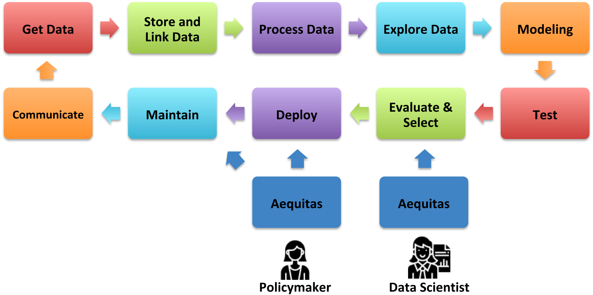
Figure 11.2: ML pipeline
Figure 11.2 puts Aequitas in the context of the machine learning workflow and shows which type of user and when the audits must be made. The main goal of Aequitas is to standardize the process of understanding model biases. By providing a toolkit for auditing by both data scientists and decision makers, it makes it possible for these different actors to take bias and fairness into consideration at all stages of decision-making in the modeling process: model selection, whether or not to deploy a model, when to retrain, the need to collect more and better data, and so on.
To get a more hands-on tutorial using Aequitas, take a look at the Aequitas Example Jupyter Notebook.
References
Adam Rose. 2010. “Are Face-Detection Cameras Racist?” http://content.time.com/time/business/article/0,8599,1954643,00.html. Accessed February 12, 2020.
Alexia Fernandez Campbell. 2018. “Women accuse Facebook of illegally posting job ads that only men can see.” https://www.vox.com/business-and-finance/2018/9/18/17874506/facebook-job-ads-discrimination. Accessed February 12, 2020.
Ali, Muhammad, Piotr Sapiezynski, Miranda Bogen, Aleksandra Korolova, Alan Mislove, and Aaron Rieke. 2019. “Discrimination Through Optimization: How Facebooks Ad Delivery Can Lead to Biased Outcomes.” Proceedings of the ACM on Human-Computer Interaction 3. New York, NY, USA: Association for Computing Machinery.
Buolamwini, Joy, and Timnit Gebru. 2018. “Gender Shades: Intersectional Accuracy Disparities in Commercial Gender Classification.” In Proceedings of the 1st Conference on Fairness, Accountability and Transparency, edited by Sorelle A. Friedler and Christo Wilson, 81:77–91. Proceedings of Machine Learning Research. New York, NY, USA: PMLR.
Celis, L. Elisa, Lingxiao Huang, Vijay Keswani, and Nisheeth K. Vishnoi. 2019. “Classification with Fairness Constraints: A Meta-Algorithm with Provable Guarantees.” In Proceedings of the Conference on Fairness, Accountability, and Transparency, 319–28. FAT* 19. New York, NY, USA: Association for Computing Machinery.
Chen, Irene, Fredrik D Johansson, and David Sontag. 2018. “Why Is My Classifier Discriminatory?” In Proceedings of the 32nd International Conference on Neural Information Processing Systems, 3543–54. NIPS 18. Red Hook, NY, USA: Curran Associates, Inc.
Chouldechova, Alexandra. 2017. “Fair Prediction with Disparate Impact: A Study of Bias in Recidivism Prediction Instruments.” Big Data 5 (2): 153–63.
Chouldechova, Alexandra, and Aaron Roth. 2018. “The Frontiers of Fairness in Machine Learning.” arXiv Preprint arXiv:1810.08810.
Conor Dougherty. 2015. “Google Photos Mistakenly Labels Black People ’Gorillas’.” https://bits.blogs.nytimes.com/2015/07/01/google-photos-mistakenly-labels-black-people-gorillas/. Accessed February 12, 2020.
Desmarais, Sarah L, and Jay P Singh. 2013. “Risk Assessment Instruments Validated and Implemented in Correctional Settings in the United States.” Lexington, KY: Council of State Governments. http://csgjusticecenter.org/wp-content/uploads/2014/07/Risk-Assessment-Instruments-Validated-and-Implemented-in-Correctional-Settings-in-the-United-States.pdf.
Drew Harwell. 2019. “San Francisco becomes first city in U.S. to ban facial-recognition software.” https://www.washingtonpost.com/technology/2019/05/14/san-francisco-becomes-first-city-us-ban-facial-recognition-software/. Accessed February 12, 2020.
Dwork, Cynthia, Moritz Hardt, Toniann Pitassi, Omer Reingold, and Richard Zemel. 2012. “Fairness Through Awareness.” In Proceedings of the 3rd Innovations in Theoretical Computer Science Conference, 214–26. ITCS 12. New York, NY, USA: Association for Computing Machinery.
Jeff Larson and Surya Mattu and Lauren Kirchner and Julia Angwin. 2016. “How We Analyzed the COMPAS Recidivism Algorithm.” https://www.propublica.org/article/how-we-analyzed-the-compas-recidivism-algorithm. Accessed February 12, 2020.
Julia Angwin and Jeff Larson. 2016. “Bias in Criminal Risk Scores Is Mathematically Inevitable, Researchers Say.” https://www.propublica.org/article/bias-in-criminal-risk-scores-is-mathematically-inevitable-researchers-say. Accessed February 12, 2020.
Julia Angwin and Jeff Larson and Surya Mattu and Lauren Kirchner. 2016. “Machine Bias.” https://www.propublica.org/article/machine-bias-risk-assessments-in-criminal-sentencing. Accessed February 12, 2020.
Julia Angwin and Terry Parris Jr. 2016. “Facebook Lets Advertisers Exclude Users by Race.” https://www.propublica.org/article/facebook-lets-advertisers-exclude-users-by-race. Accessed February 12, 2020.
Kilbertus, Niki, Mateo Rojas Carulla, Giambattista Parascandolo, Moritz Hardt, Dominik Janzing, and Bernhard Schölkopf. 2017. “Avoiding Discrimination Through Causal Reasoning.” In Advances in Neural Information Processing Systems 30, 656–66. Curran Associates, Inc.
Kleinberg, Jon, Sendhil Mullainathan, and Manish Raghavan. 2017. “Inherent Trade-Offs in the Fair Determination of Risk Scores.” In 8th Innovations in Theoretical Computer Science Conference (ITCS 2017), edited by Christos H. Papadimitriou. Vol. 67. Dagstuhl, Germany: Schloss Dagstuhl–Leibniz-Zentrum fuer Informatik.
Kusner, Matt J, Joshua Loftus, Chris Russell, and Ricardo Silva. 2017. “Counterfactual Fairness.” In Advances in Neural Information Processing Systems 30, 4066–76. Curran Associates, Inc.
Lambrecht, Anja, and Catherine Tucker. 2019. “Algorithmic Bias? An Empirical Study of Apparent Gender-Based Discrimination in the Display of Stem Career Ads.” Management Science 65 (7): 2966–81.
Rodolfa, K., E. Salomon, L. Haynes, I. Mendieta, J. Larson, and R. Ghani. 2020. “Predictive Fairness to Reduce Misdemeanor Recidivism Through Social Service Interventions.” In Proceedings of the ACM Conference on Fairness, Accountability, and Transparency (ACM FAT*) 2020.
Russell Brandom. 2019. “Facebook has been charged with housing discrimination by the US government.” https://www.theverge.com/2019/3/28/18285178/facebook-hud-lawsuit-fair-housing-discrimination. Accessed February 12, 2020.
The Northpointe Suite. 2016. “Response to ProPublica: Demonstrating accuracy equity and predictive parity.” https://www.equivant.com/response-to-propublica-demonstrating-accuracy-equity-and-predictive-parity/. Accessed February 12, 2020.
Zafar, Muhammad Bilal, Isabel Valera, Manuel Gomez Rogriguez, and Krishna P. Gummadi. 2017. “Fairness Constraints: Mechanisms for Fair Classification.” In Proceedings of the 20th International Conference on Artificial Intelligence and Statistics, edited by Aarti Singh and Jerry Zhu, 54:962–70. Proceedings of Machine Learning Research. Fort Lauderdale, FL, USA: PMLR.
Zemel, Rich, Yu Wu, Kevin Swersky, Toni Pitassi, and Cynthia Dwork. 2013. “Learning Fair Representations.” In Proceedings of the 30th International Conference on Machine Learning, edited by Sanjoy Dasgupta and David McAllester, 28:325–33. Proceedings of Machine Learning Research 3. Atlanta, Georgia, USA: PMLR.